The leading regular perturbation equation has . Its homogeneous solutions are and , soThe boundary data must also be expanded: , while the right endpoint value is independent of . Thus and , givingSince , the unique values are , . ThereforeIts derivatives are and , so the leading differential equation and both leading endpoint values can be checked directly.
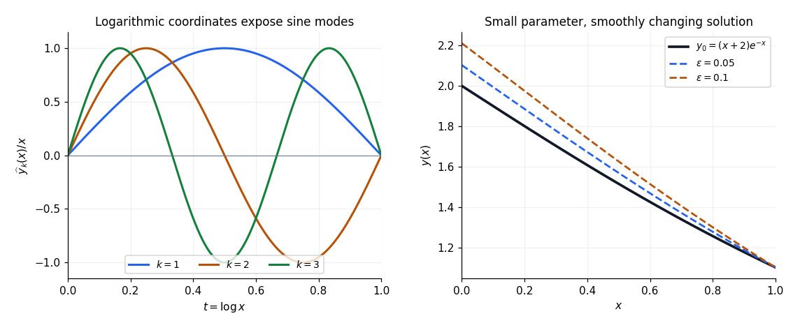
Logarithmic eigenmodes and the leading regular perturbation solution
. The left panel shows three eigenfunctions after division by x and the change of variable t = log x. The right panel compares the derived leading term with numerical boundary value solutions at two small parameter values; these are original calculations. Details.
Let . Matching powers in the regular perturbation expansion and in the Taylor series of the left endpoint value gives the complete recursive boundary value problemThe higher-order left endpoint values are not zero. The parameter-dependent boundary data in a regular perturbation hierarchy rule applies here.
First prove uniqueness for any one of these forced problems. The difference of two solutions obeys and homogeneous Dirichlet boundary conditions. The positive integrating factor givesMultiplication by and integration by parts yieldHence , and the endpoint values force . The kernel is trivial: zero is not an eigenvalue of this homogeneous Dirichlet boundary value problem.
Existence is also explicit. For arbitrary smooth forcing and endpoint values , , two integrations of givewhereSince , the unique choicealways meets the second endpoint value. Starting from the smooth , induction with , , proves existence and uniqueness at every order.
Equivalently, the Fredholm alternative has no compatibility obstruction because the homogeneous kernel vanishes; the corresponding adjoint operator has no zero eigenvalue either. The direct construction above proves this without computing any particular beyond the leading term.
Articles by others on the same topic
There are currently no matching articles.