Solutions to all three questions of the University of Oxford Differential Equations II paper, sat on 22 June 2023. Source: released examination PDF, parent PDF pages 118–120; questions on pages 119–120. Question statements are omitted. In Question 2(b), the usual interpretation that the forcing extends continuously to the closed interval is distinguished from continuity only in the interior.
The characteristic equation of the linear ordinary differential equation is , with roots . A real pair of homogeneous solutions is thereforeTheir Wronskian, with the convention , isThus the two functions are linearly independent throughout the interval and span its homogeneous solutions.
Use the unweighted inner product . Two applications of integration by parts giveThe given boundary conditions set at both ends, but leave and independently variable. The remaining boundary term vanishes for every admissible precisely when . Consequently the formal adjoint and the boundary conditions specifying the adjoint operator are
Set . To construct the Green's function from a Dirac delta function, require and zero endpoint values. Away from , the homogeneous solutions satisfying the left and right boundary conditions are respectivelyWrite for and for . A discontinuity in would generate a derivative of the Dirac delta function, which is absent from the desired equation. Thus is continuous. Integrating that equation through then gives the jump conditionThe resulting two equations are and . Since the Wronskian , they giveBoth endpoint values vanish. At , subtracting the two first derivatives gives , verifying the sign and normalization of the Dirac delta function.
The homogeneous solution already has the prescribed endpoint values. Thus has zero boundary conditions and satisfies . The Green's function givesEquivalently, splitting the integral at gives the explicit formulaAny difference between two solutions would be with zero endpoint values, forcing . The displayed solution is therefore unique.
At , the nonzero homogeneous solution satisfies both zero boundary conditions. Thus the boundary value problem has a nontrivial kernel and cannot have an inverse for arbitrary forcing.
More directly, the adjoint operator has the zero-endpoint homogeneous solution . If an ordinary Green's function existed, the integration by parts identity would implyBut for . This contradiction rules out the Green's function for the unmodified operator. It is the Fredholm alternative obstruction.
The nonzero endpoint data contribute to the Fredholm alternative condition. With , the same integration by parts identity givesFor the specified forcing the left side is . HenceTo verify sufficiency, set . Direct differentiation gives . At this value of , a particular solution of is . The complete family obeying the two boundary conditions isThe arbitrary constant records the one-dimensional kernel; existence does not imply uniqueness here.
Put . After division by , the Legendre differential equation has coefficientsBoth are analytic functions at zero, so . At either , has a genuine simple pole; hence these are singular points even when makes vanish. However,and both products extend analytically across . By the regular singular point criterion for a second-order equation,None of the three specified points is an irregular singular point.
Use . The Legendre differential equation becomesSubstituting a Frobenius series , , gives the indicial equation : the indicial root zero is repeated. For , the coefficient of yieldsorFor the multiplying factor is nonzero. At it vanishes, so and all later coefficients are zero. Thus one solution is a polynomial of exact polynomial degree , including a nonzero constant when . Denote a chosen normalization by .
The linear recurrence relation determines every analytic coefficient from , so there cannot be a second independent analytic solution at . To see the required logarithm explicitly, reduction of order gives the second solution locally asNear , the integrand is plus an analytic function. After rescaling the second solution, its form is thereforeThe analytic remainder converges locally; its constant term may be set to zero by adding a multiple of . The nonzero logarithmic coefficient makes linearly independent of . This Frobenius expansion of the Legendre equation at an endpoint gives a Logarithmic Frobenius solution; the same endpoint calculation at explains why the independent Legendre function of the second kind is excluded when boundedness at both ends is required.
Write the operator in divergence form:The Legendre differential equation therefore givesThese are the eigenvalues of . With the common positive-sign convention for a Sturm-Liouville problem, use instead:This is a singular Sturm-Liouville problem, because vanishes at the endpoints. Bounded eigenfunctions select the nonlogarithmic branches and satisfy there. The Lagrange identity for a Sturm-Liouville operator givesThe eigenvalues are distinct, proving the orthogonality conditionThe weight is one. No choice of normalization of the Legendre polynomials is needed for this conclusion.
First take the usual endpoint-regular interpretation . Integrating the divergence form shows that has finite endpoint limits. A nonzero limit would make proportional to near that endpoint, forcing a logarithmically unbounded . Thus boundedness requires , and consequentlyThis is orthogonality to the constant eigenfunction , hence the Fredholm alternative condition. It is also sufficient under the stated endpoint regularity: putIf , the zero-mean condition gives . Hence the last integrand is bounded, so extends continuously to both endpoints. Any two bounded solutions differ by a constant: their difference solves , whose other solution is .
For the requested eigenfunction expansion, setThe Legendre polynomials span all polynomials, so their completeness follows from the Weierstrass approximation theorem. Projecting onto each eigenfunction gives for . The zero mode is free, while . Thus the full family isThe formula is unchanged by rescaling any . For the usual normalization , the facts on and , together with the Cauchy-Schwarz inequality, bound each summand by a constant times . The series therefore converges absolutely and uniformly. Its identification with the preceding integral solution avoids unjustified termwise second differentiation.
There is a source ambiguity: continuity only on does not supply the endpoint control used above. Even for integrable forcing, zero mean alone is insufficient. For example, letThis is continuous in the interior, absolutely integrable, and has zero mean because . Yet every candidate with zero endpoint values of haswhose integral diverges logarithmically in at each endpoint. Thus no bounded solution exists. For a merely interior-continuous , the exact criterion is that some constant makesbounded as approaches both endpoints. The Bounded solvability for the Legendre operator criterion above covers the intended regular forcing and makes this endpoint limitation explicit.
When , the forcing has nonzero integral , violating the Fredholm alternative condition. There is no bounded solution. Directly, integration gives ; cancellation of its logarithmic divergence at requires , while cancellation at requires .
For , the constant is a particular solution. Subtract it from any solution. The remainder satisfies the Legendre differential equation, whose general solution is a combination of and the logarithmically unbounded Legendre function of the second kind. Boundedness removes the latter coefficient, givingThe constant forcing is orthogonal to for , consistently with Orthogonality of Legendre polynomials and the Fredholm alternative.
Consider real roots. Every zero at is , , and its derivative is nonzero. For a regular perturbation, write . The Taylor seriesgives . Thus, through the requested order,There is no quadratic term. The exact parametrization also verifies completeness and the remainder order for .
Take . There are two real branches, on different scales. For a root tending to zero, the Taylor series givesThe dominant balance is , so a fractional-power root expansion yieldsMore precisely . An ordinary power series in integer powers of would miss this scale.
There is also a root escaping to positive infinity. Boundedness of the sine term makes the leading dominant balance . The nonzero branch isIndeed the equation rearranges to , which yields on this branch. The bounded oscillatory correction need not have a constant limiting value.
To check that these are all the real solutions, solve for the parameter:Positive values occur only on and ; are not roots. A useful exact derivative isIt vanishes only at isolated points, so is strictly decreasing on each of these intervals. Its endpoint limits are and zero on each interval. This monotone parametrization of sine perturbation roots gives exactly one root in each interval for every , proving that both asymptotic branches, and no others, have been included. If negative small parameters are allowed, the transformation reflects these two branches and gives all real solutions for that sign as well.
For the positive coefficient of , setting gives the reduced equation , with general solution . A fast decaying homogeneous solution of is , placing the boundary layer at the left endpoint. Thus use the right boundary condition for the outer solution: impliesThe dominant balance gives width . With the inner variable and , the exact rescaled equation isAt leading order, , so . The asymptotic matching condition sets , and sets . ThereforeThe additive composite expansion has zero overlap to subtract. Its graph starts at one, decreases steeply over , and then stays close to zero; its initial slope is . The right endpoint discrepancy is exponentially small. The left panel of the figure below sketches this profile. A right-end inner expansion would instead contain a growing term and could not repair the left endpoint mismatch.
With the negative coefficient of , the reduced equation is unchanged, but the fast mode now decays away from the right endpoint. Apply the left boundary condition to the outer solution, givingThe boundary layer still has width . Put and . The rescaled equation isIts leading inner expansion has . The asymptotic matching condition is , while . ThusSubtracting the overlap in the additive composite expansion givesIts graph starts exponentially close to one, follows the gently decreasing outer solution, and drops from near to zero in a right boundary layer of width . The right endpoint value is exactly zero; the left endpoint error is . Its right endpoint slope is , showing the rapid final descent.
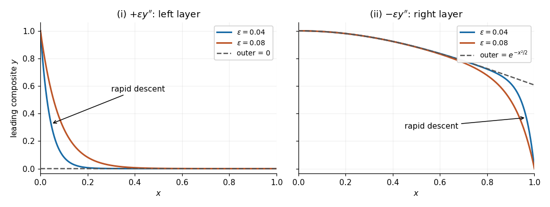
Leading composite profiles for the two signs of the highest derivative
. Original sketches from the derived additive composite expansions, for and . Left: the positive sign gives a left boundary layer and zero outer solution. Right: the negative sign gives a right boundary layer and the outer solution . Dashed curves show the corresponding outer solutions. Details.
Solutions to all three questions of the University of Oxford Differential Equations II paper, sat on 25 June 2021. Source: released examination PDF, bundle pages 111–113; questions on pages 112–113.
Take and use the inner product on the Hilbert space . The differential operator has domainwhere is a Sobolev space. Twice applying integration by parts gives the Lagrange identity for a Sturm-Liouville operatorThe Dirichlet boundary conditions make this expression zero for , and the formal adjoint is . To obtain the domain of the adjoint operator, initially impose the boundary conditions only on . The remaining expression is . Since and vary independently, it vanishes for all such exactly when . The adjoint domain is therefore the original domain: this is full self-adjointness, including the boundary conditions.
Consequently the eigenvalues are real, eigenfunctions for distinct eigenvalues are orthogonal, and regular Sturm-Liouville theory supplies a complete orthonormal eigenbasis. Here these objects can be exhibited explicitly:Indeed , and the Fourier sine basis is complete in . There are no additional eigenvalues: for a nonzero eigenfunction , integration by parts givesso and the endpoint values force . All these eigenvalues are simple. The eigenvectors are precisely the nonzero multiples of these eigenfunctions, regarded as vectors in the Hilbert space.
The homogeneous solution is . The left boundary condition removes , and the right boundary condition gives . Thus the kernel of a linear map associated with this boundary value problem isThe Fredholm alternative now gives the complete classification:For necessity at , multiply by the homogeneous solution and use the Lagrange identity for a Sturm-Liouville operator to obtain . For sufficiency, the particular solutionsatisfies and . At the other endpoint,which is zero under the compatibility condition. All solutions are then , with arbitrary. The assumed Lipschitz continuity of in particular makes continuous, so the displayed integral defines a classical solution. The length is excluded: it would not define a nonempty interval for this boundary value problem.
For , use variation of parameters with the homogeneous solutions , whose Wronskian is one. Write and impose . The differential equation gives , henceAfter integrating from zero and using the left boundary condition,The right boundary condition determinesso the unique solution isCombining the two integrals gives , with Green's functionIt is symmetric in , as expected from self-adjointness, and has zero endpoint values. At it is continuous, while its first derivative obeys the jump conditionThus , with the positive normalization of the Dirac delta function required for .
Expand in the Fourier sine basis, using unnormalized eigenfunctions:Projection of onto each eigenfunction givesWhen , every eigenvalue is nonzero and the eigenfunction expansion is uniquely determined:When , the exceptional index is , for which the eigenfunction is . If , its coefficient equation is , an inconsistency: there is no solution. If , the coefficient equation is , and is arbitrary. The full family isThis is the Fredholm alternative directly in the coefficient equations: nonzero eigenvalues fix their coefficients; a zero eigenvalue requires zero forcing in that direction and leaves the corresponding coefficient free. An inconsistent equation at a zero eigenvalue cannot be repaired by assigning an infinite coefficient.
For convergence, Lipschitz continuity implies absolute continuity of , with bounded derivative almost everywhere. One integration by parts gives ; since the denominators grow quadratically, apart from the single free coefficient. The solution series and its first derivative therefore converge uniformly. The second derivative converges in , and the resulting Sobolev space solution satisfies . As is a continuous function, this is a classical solution, with both boundary conditions satisfied. The forcing's Fourier sine series is interpreted on the open interval or in ; its endpoint values need not equal the endpoint values of .
At , the Fredholm solvability condition isby orthogonality of the Fourier sine basis. Thus a non-unique solution exists exactly when , with any real . Since , the complete family isIf there is no solution, for any . In particular, when , the family reduces to the kernel ; it is still non-unique. There is no choice of producing a unique solution for this length.
Putting both data at zero makes this an initial value problem. The uniqueness theorem for ordinary differential equations applies, and one can also prove uniqueness directly: the difference of two solutions is a homogeneous solution whose value and first derivative at zero are both zero, forcing . In fact, for every prescribed continuous function ,satisfies both initial data and . Consequently non-uniqueness is impossible for every , including . In this setting the kernel is trivial. The boundary conditions at a single endpoint do not give the same self-adjoint operator domain as the two separated Dirichlet boundary conditions, so the earlier exceptional lengths do not apply.
Work first on . For , the power-law ansatz gives the indicial equation . Therefore the Cauchy-Euler equation has general solutionFor the repeated indicial root supplies the logarithm rather than two copies of the constant solution. Alternatively, the change of variables turns the differential equation into . On the corresponding real formulas use and , with independent constants on the two sides of zero.
For general , normalize the second-order linear differential equation asThe coefficient is singular at zero, but and are analytic functions there because is a positive integer. The regular singular point criterion for a second-order equation therefore proves that zero is a regular singular point for every allowed . The indicial equation remains .
For the first Frobenius solution, take the larger indicial root and normalize the first coefficient to one:Substitution and comparison of the coefficient of giveEvery denominator is nonzero because .
For , the recurrence relation is , soFor , and all odd coefficients vanish; the even coefficients satisfy . HenceFor any positive integer , induction in the recurrence relation shows that only indices divisible by survive:The empty product for equals one. Successive terms in the power series factor have ratio of magnitudesThus the ratio test gives convergence for every finite ; a nonintegral still requires a chosen side of zero or a complex branch for the factor .
For a putative second Frobenius solution with the smaller indicial root , set , with and for . Its recurrence relation isThe Frobenius case classification concerns the gap between the indicial roots. In the course convention, Case IIIa is the obstructed recurrence requiring a Logarithmic Frobenius solution; Case IIIb permits two pure Frobenius series.
If and , this is Case I: no denominator vanishes. There are two linearly independent pure Frobenius solutions, withTheir different leading powers establish linear independence.
If , this is Case II, with a repeated indicial root. There is only one pure Frobenius series with a nonzero leading coefficient. To see the second solution's form, reduction of order givesHere , so the integrand is . ConsequentlyThe logarithm has a nonzero coefficient and cannot be removed by adding a multiple of .
If is a positive integer, the only potentially obstructed coefficient is . Below that index, unless divides . At the exceptional index the equation readsIf for some positive integer , all coefficients are nonzero because . The exceptional equation is inconsistent. This is Case IIIa, and the independent second solution has the formThe Frobenius resonance for an Euler equation with monomial potential explains why divisibility, rather than the integer gap alone, decides this outcome. For example, with , applying the original differential operator to gives . Cancellation of the coefficient of requires .
If does not divide , then ; this includes through the negative-index convention. The exceptional equation is , so is free. This is Case IIIb: set to select an independent pure Frobenius series starting with . Subsequent coefficients again follow the recurrence relation. Changing simply adds a multiple of , the undetermined coefficient at Frobenius resonance.
The complete answer is thereforeIn particular, for every positive integer gap gives Case IIIa. For , positive integer gives Case IIIa, while gives Case IIIb; the remaining positive give Case I. The condition matters: at the two Cauchy-Euler equation powers already give independent solutions whenever .
Normalize both leading coefficients to one. For the indicial root , the recurrence relation from part (b) givesRecognizing the Taylor series of the sine gives the first Frobenius solutionFor the smaller indicial root , . The equation at is ; choose the free coefficient to avoid adding the first Frobenius solution. The remaining coefficients areThus the Taylor series of the cosine givesTheir leading terms are and , as required for Case IIIb. A direct check uses : the differential equation becomes , so these two functions solve it on . Their Wronskian is , proving linear independence. The general solution is .
The function is an odd function, passes through , and has the horizontal asymptote at both infinities. Its derivative isIt decreases for and increases for , with its lowest value and highest value . These features determine the graph of a function shown below.
For , the equation is the quadratic equation . The quadratic formula gives exactly two real equation roots:The binomial series gives , hence the two requested asymptotic expansions areTheir product is exactly one. Both are positive, with ; there are no negative equation roots because for . At the two real equation roots coincide at one, and for there are none. In the stated limit , these two branches are therefore exhaustive.
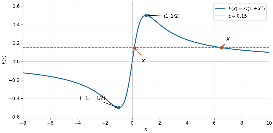
Two positive intersections of the rational function with a small positive level
. Original sketch of with the two real equation roots marked for . The curve also shows its negative lowest point and positive highest point. Details.
The power-law ansatz givesSince , the equation roots and are distinct. The Cauchy-Euler equation therefore has general solutionFor , the first derivative and second derivative areThe strictly convex function diverges to as , passes through , and has a unique lowest point atAs , , so the line is an asymptote. When , the lowest point is to the right of one; at it is at one, and for it is to the left of one.
The ratio of the two terms isThus is larger for , the terms are equal at , and is larger for . In the stronger asymptotic sense as , dominates at each fixed , and dominates at each fixed . Their crossover has , equivalently , as described by the power-law crossover in a singular perturbation. In that region with bounded gives .
Substitute the proposed regular perturbation into the differential equation. The leading and subsequent equations areConsequently , and in fact each successive coefficient has the form , because the preceding second derivative is zero. The leading approximation is thereforeIt has only one adjustable constant and generally cannot impose two independent boundary conditions. Those assumed in the question require a nonzero coefficient, which a power series in cannot recover: at fixed it is exponentially small, and at fixed it grows without bound as . Thus the regular perturbation describes the specified solution only in the region to the right of the crossover, away from ; it is not a uniform approximation on .
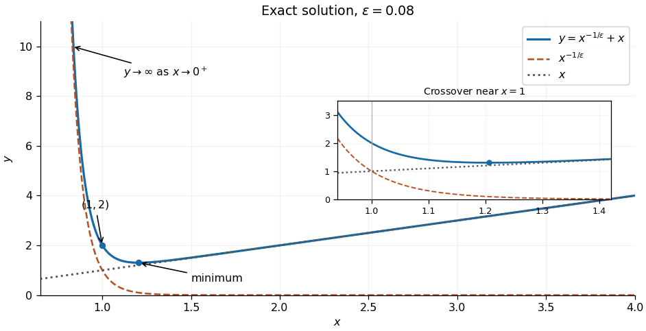
The exact solution and its two power-law contributions
. Original sketch for , showing the decreasing contribution, the increasing contribution, their sum, and its lowest point. The inset resolves the region where both terms contribute. Details.
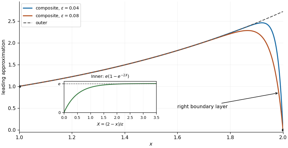
Setting gives the reduced first-order linear differential equation . Its nonzero solutions cannot satisfy the zero value at , so one endpoint needs a boundary layer. To determine which endpoint, freeze the coefficient at in the rapidly varying part: has fast mode . It decays into the interval from the right endpoint but grows into the interval from the left endpoint. HenceThe dominant balance gives , so a convenient local thickness is . The left boundary condition must select the outer solution. Equivalently, a putative left inner variable would give , whose nonconstant solution grows like and cannot satisfy the asymptotic matching condition as .
The reduced equation and the left boundary condition give the leading outer solutionIntroduce the right inner variable and write . The chain rule gives and . Multiplying the rescaled differential equation by gives the exact equationAt leading order, , with general solution . The right boundary condition gives . The asymptotic matching condition in the overlap region givesThus and , yielding the leading inner expansionEquivalently, the inner variable gives . Both normalizations describe the same boundary layer.
The common value in the overlap region is . The additive composite expansion therefore givesThis leading approximation has and ; the left endpoint error is exponentially small. It rises from near one following the outer solution , approaches a value close to , then drops rapidly to zero in the right boundary layer. Its first derivative isFor small the largest value lies slightly inside the interval. For this additive composite expansion, the first derivative vanishes atThis locates the rounded top of the sketch; the rapid final drop has the scale found above. The additive composite expansion is a leading approximation, so its exponentially small endpoint error does not imply an exponentially small error throughout the interval: neglected algebraic corrections to the outer expansion and inner expansion remain.

Source paper: released examination archive, member
2016/T/a13758w1.pdf. The original cover dates this examination to 2017-06-23.The complete four-page replacement is in the Mathematics Part A FOI release, member
FOI-20210708-1 - Data/a13758w1 (2).pdf. Its cover confirms the same A6 paper, formal code A13758W1, sitting on 23 June 2017. This copy supplies the previously missing printed pages 3–4; the original source above is retained for provenance.Extend the given functions continuously to zero by . This is forced by their stated differentiability. Their derivatives at zero are both zero, since the corresponding difference quotients tend to zero.
For , , and for , . At zero all four quantities vanish. Thus the Wronskian isNevertheless, if the constant linear combination vanishes identically, evaluation at gives , and evaluation at gives . Therefore the two functions are linearly independent.
This illustrates why a vanishing Wronskian does not imply linear dependence for arbitrary differentiable functions. Here both functions are continuously differentiable, but neither has a second derivative at zero. The common regular differential equation hypothesis in the next part is absent.
Differentiate the Wronskian using the product rule and substitute the common homogeneous linear differential equation:Multiplying this first-order equation by the integrating factor and integrating gives Abel's identity:The exponential factor is finite and nonzero for every in the given interval, because is continuous on the compact interval between and . Hence implies everywhere in that interval. Using an integrating factor avoids dividing by , which would assume the conclusion.
Interpret the Dirac delta coefficient as a point interaction in a second-order differential equation. The solution is continuous at and is twice differentiable on either side, where . Its transmission conditions for a delta coefficient areIndeed, the distributional second derivative across a jump contributes , which must cancel the delta coefficient because has no point source.
Put and . Integrating the ordinary equation and inserting the required derivative jump giveswhere . This formula is continuous, has the stated jump, satisfies the equation, and parametrizes every solution with the left endpoint value. Imposing the right endpoint value gives the scalar equationConsequently a unique , and hence a unique solution for every , exists precisely whenAt the exceptional value, the nonzero homogeneous solution with zero endpoint values isIt has derivative jump . Thus uniqueness fails. More precisely, there are infinitely many solutions ifand none otherwise. This follows either from the scalar equation or by integration by parts against . It is the compatibility obstruction at Dirichlet resonance for a point interaction.
Use a Green function satisfying with homogeneous Dirichlet boundary conditions , for . Since away from and , it is continuous and piecewise affine, with possible derivative jumps at those two locations.
For , the transmission conditions for a delta coefficient and the unit source condition areIf , there is a single junction, and the correct combined condition isFor example, a suitable piecewise form when iswhere the coefficients depend on . The two continuity conditions, and determine them. When , use the same affine form on the intervals cut at , with and instead. This gives all requested boundary and jump conditions without needing the coefficients.
An explicit compact kernel also makes the construction transparent. The left and right homogeneous solutions at areThey obey the interaction jump and have Wronskian on either side. ThereforeDifferentiating its two branches at the source gives a unit derivative jump whenever . At , and , so the combined condition is also satisfied. This is the Dirichlet Green function for a point interaction specialized to the present parameters.
The Green kernel itself has zero endpoint values. The prescribed nonzero endpoint values enter through the homogeneous lift:Indeed, and . The kernel accounts for the forcing; the lift accounts for the boundary data. Uniqueness follows from part (i), since .
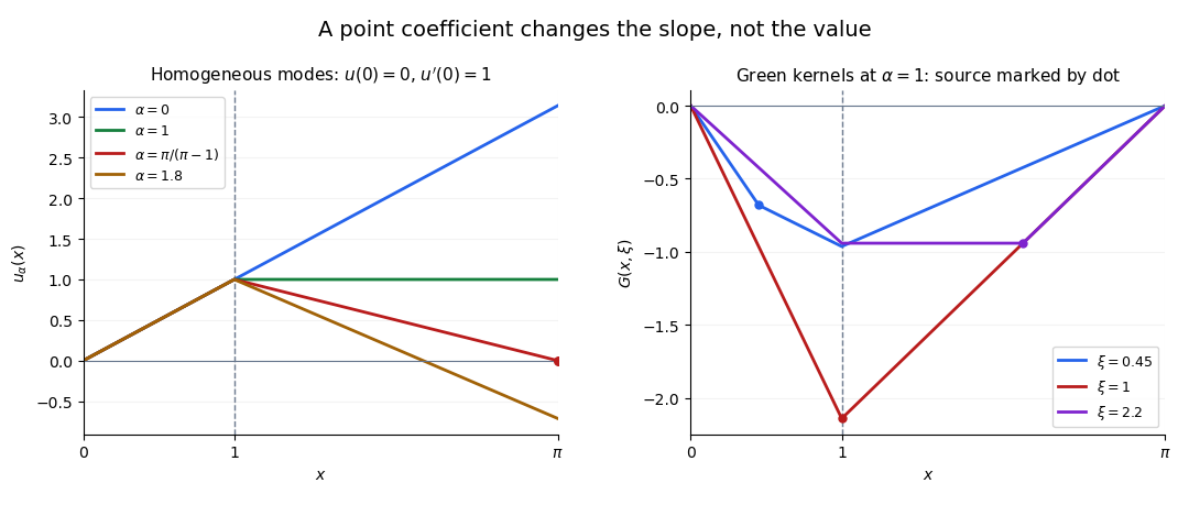
The resonant homogeneous mode and the derivative jumps of the Green kernel
. Original calculations for an interaction at on . The left panel varies the coefficient with a fixed initial slope; the resonant curve alone meets the zero right boundary. The right panel shows three source positions at coefficient one, including a source coinciding with the interaction. Details.
Use integration by parts with a complex conjugate, so that the argument also covers complex-valued eigenfunctions. The coefficient functions are understood to be real. For a nonzero eigenfunction with Dirichlet boundary conditions,The denominator is strictly positive and the numerator is real. Consequently the eigenvalue satisfiesThis is the Rayleigh quotient for the sign convention used here. Positivity of is unnecessary for this particular reality argument; real coefficients and disappearance of the endpoint term are what matter.
The Lagrange identity for a Sturm-Liouville operator givesIn the intended class of functions whose values and first derivatives stay finite at the endpoints, the endpoint factor makes this entire boundary term vanish. Thus no separately prescribed endpoint values are needed to eliminate the boundary form. The same integration by parts argument then proves that the eigenvalues are real.
The admissible endpoint behaviour is part of this conclusion: it is the vanishing endpoint coefficient and the Sturm-Liouville boundary form, together with endpoint regularity, that replaces explicit boundary conditions. If singular functions are allowed, a vanishing coefficient alone need not suffice: and have as . A self-adjoint differential operator therefore still needs a specified domain of admissible functions.
Articles were limited to the first 100 out of 165 total.
Articles by others on the same topic
There are currently no matching articles.