The strongest evidence for large-scale cosmological isotropy is the nearly direction-independent blackbody temperature of the cosmic microwave background. After removing the dipole associated mainly with our peculiar velocity, its residual temperature fluctuations are of order . Nearly isotropic counts of distant radio sources and galaxies, after correcting for sky coverage and selection effects, provide independent evidence. Local galaxies, clusters and voids clearly are not isotropic structures; the claim concerns a statistical description on sufficiently large scales.
Large redshift surveys show that the mean galaxy density stabilizes as increasingly large volumes are sampled, and that the excess pair correlations weaken at large separations. This supports statistical homogeneity beyond the characteristic clustering scales. The consistency of large-scale observations in different directions and the success of a common FRW metric description are additional checks.
Isotropy around one observer does not alone prove spatial homogeneity: a radially varying distribution centered on that observer could look isotropic. The Copernican principle supplies the assumption that we occupy no preferred position; comparable isotropy about typical locations then supports the cosmological principle. Surveys observe a finite past light cone, with source evolution and selection, so they cannot establish homogeneity everywhere on a simultaneous spatial slice. The evidence supports large-scale statistical isotropy and homogeneity, with substantial small-scale structure and an explicit typical-observer assumption.
Use a radial null geodesic of the FRW metric in the form along a fixed spatial direction, with . For an emitter and observer at fixed comoving coordinates, the comoving separation isApply this to two adjacent wave crests. Since their endpoint separation is the same, subtraction to first order gives . These intervals are the local periods measured by the comoving observers, so the received wavelength is stretched by . Consequently the cosmological redshift obeyswhen . This relation assumes comoving emitter and observer; additional peculiar velocities supply kinematic redshift factors.
A comoving coordinate labels a location in the expanding background and is constant for an object moving with the Hubble flow. For example, a radial comoving geodesic coordinate gives proper distance in cosmology along the constant-cosmic-time slice. In a flat background one can write physical coordinates and split the physical velocity asThus proper distance in cosmology is measured using the spatial metric at a specified epoch, whereas a comoving distance factors out the overall expansion. A proper distance on a simultaneous spatial slice is not automatically the luminosity distance or a distance directly inferred from light received today. In a curved spatial geometry is the radial proper distance, while the sphere's circumference involves the corresponding curved radial function.
The Friedmann acceleration equation gives the gravitational deceleration from a uniform pressureless matter density, plus the acceleration from a cosmological constant. Here is the matter mass density, is the gravitational constant, is the Hubble parameter, and is the constant spatial-curvature coefficient in the chosen normalization of . The Friedmann equation is the first integral relating expansion to density, curvature and vacuum energy. With , the matter, curvature and cosmological-constant contributions to are , and . The cosmological constant has effective density and equation-of-state parameter ; its negative pressure explains its positive acceleration contribution when .
For the Newtonian derivation with , follow a test mass on the edge of a uniform sphere of physical radius . Conservation of the enclosed matter gives constant. The shell theorem removes the force of external spherical shells and givesIntegrating the force equation once gives the conserved specific mechanical energyDivide by to obtainHomologous motion makes constant between shells. Newtonian mechanics supplies this energy integration constant; its interpretation as intrinsic spatial curvature belongs to the relativistic FRW metric.
An outward acceleration comes from the Newtonian potential per unit masssince . With conventional dimensional , restore in this potential and the corresponding acceleration and Friedmann terms.
A genuine nondegenerate bounce has and ; using also includes the limiting stationary case. Put , and define the present matter density parameter , and . The dust-plus-cosmological-constant Friedmann equation and its acceleration equation becomeAt the bounce these giveFor a past bounce with , eliminate from the first equation:Subtracting and multiplying by the positive denominator givesThus the matter bound from a Friedmann bounce isStrict positive bounce acceleration makes this inequality strict. The zero of the Friedmann equation also requires positive curvature for positive matter and positive .
An observed source at has . Since the minimum scale factor cannot exceed the scale factor at emission, . The denominator of the bound increases with positive , soThe observational lower bound is much larger. Cluster mass-to-light ratios, inferred independently from motions, gas temperatures and gravitational lensing, combined with the observed luminosity density imply substantial cosmic mass density. Measurements of the cosmic baryon fraction from representative clusters, combined with the baryon cosmological density parameter inferred from Big Bang nucleosynthesis, provide another estimate: . Large-scale clustering and peculiar velocities provide independent dynamical checks, although their interpretation must account for galaxy bias. These methods support matter densities of order a few tenths, rather than below one percent. The dust-plus-cosmological-constant bouncing model is incompatible with both a quasar at redshift six and the stated observational evidence for .
For a flat universe containing only the stated fluid, the cosmological continuity equation is . A constant equation-of-state parameter therefore gives . Combine this with the Friedmann equation to findOn the expanding branch, specifying yieldsThe solution is used only where its denominator is positive. For , integration also givesFor , choosing the zero of time at the initial singularity gives and . For , , is constant and . For , the displayed initial-value solution instead grows towards a future finite-time singularity; it is not the ordinary positive-time Big Bang branch. With positive density, accelerated expansion requires .
Adding and subtracting the canonical scalar field density and pressure givesA real scalar with positive kinetic energy consequently needs . On the expanding scalar-dominated branch, divide by and use the Friedmann equation:Choose the positive rolling sign. Integration and elimination of using give the scalar-field reconstruction for a constant equation of state:Changing the rolling sign reverses the exponential slope. At , is constant and ; elimination by an invertible then degenerates. The cosmological continuity equation gives whenever , so the reconstruction satisfies the field equation as well as the Friedmann equation.
Compare the reconstructed exponent with . In this constant-, scalar-dominated scaling solution,Strict requires , and acceleration requires . HenceThe accelerating branch has . The zero-slope limit is a constant potential with , so it does not meet the strict inequality. This result characterizes the exponential-potential power-law inflation solution; an arbitrary trajectory with the same potential need not have constant throughout its evolution.
For equal intrinsic bolometric luminosities , the observed fluxes are . In the flat model, a null geodesic gives the comoving distance . Photon energies and arrival rates each bring one factor of , yielding the luminosity distance . ThusFor the one-component constant- universe, . Its luminosity distance iswith the continuous limit for . Measurements spanning several redshifts fit the shape of this relation and hence ; the common luminosity and cancel in the flux ratio. Equivalently, the relative distance modulus is .
Actual Type Ia supernovae are standardized through their light-curve shape and color rather than being identical standard candles. Scatter, dust extinction, changes in progenitor populations, photometric calibration, spectral corrections between observed bands, flux-limited selection, lensing magnification and low-redshift peculiar velocities all affect inferred distances. The assumed cosmological model is another uncertainty: with a separate matter component, in the flat case, so is partly degenerate with ; allowing spatial curvature or varying adds degeneracies. Flux ratios constrain the expansion history through an integral of , rather than measuring directly without model assumptions.
For pressureless matter with curvature and a possible constant cosmological constant, write the background Friedmann equation asDifferentiating on the expanding branch givesConsequentlyThis proves that the Hubble parameter as a solution of the dust growth equation is valid, including constant- and curvature contributions to the background. It does not extend without change to a radiation background or arbitrary dynamical dark energy.
In an Einstein-de Sitter universe, , and . The linear matter perturbation growth equation becomesSubstitute . The indicial equation is , with roots and . ThereforeThe Hubble-parameter solution is the decaying mode in the Einstein-de Sitter universe.
Choose the Fourier transform conventionStatistical homogeneity makes the Fourier covariance diagonal, and isotropy makes the matter power spectrum depend only on . The two-point correlation function follows by inserting the transform and using this covariance:Integrating the polar angle relative to gives . HenceThe inverse isotropic transform is whenever these transforms exist, with distributions or regularization otherwise.
For a spherical average of comoving radius , the spherical top-hat window function isAt a fixed epoch let . The scale-free smoothed density variance isThus the RMS fractional mass fluctuation scales as ; the RMS mass fluctuation itself scales as at fixed epoch.
The comoving Poisson equation gives . For the growing irrotational mode the linearized cosmological continuity equation gives , where . The averaged-potential and bulk-velocity variances are thereforeFor a single Cartesian component of the isotropic bulk velocity, divide its variance by three. Rescaling givesThese are dimensional scaling laws, with an important convergence qualification. Since at small and has large- envelope , the density average converges for , the absolute potential average for , and the bulk velocity for . No one unbroken power law makes all three absolute averages finite on the entire range . In particular, long-wavelength modes can dominate the potential. Physical infrared/ultraviolet cutoffs, potential differences, or fluctuation amplitudes in a band around resolve the relevant divergences; with cutoffs the simple powers need not describe the full integrated variance. The scale-free potential and bulk-flow variance laws should be understood with these conditions, not as a claim that divergent RMS integrals are finite.
Use the same negative-exponent Fourier transform as in the preceding part and let . In linear theory, , and the linearized cosmological continuity equation is . Its irrotational solution isHere labels the comoving spatial position for the Fourier expansion. The quantity being differentiated is also , by the Poisson equation; thus this explicitly obtains the velocity from the Fourier components of the peculiar gravitational potential.
Conjugating the Rayleigh plane-wave expansion, and using the symmetric addition formula for spherical harmonics, givesFor the radial component , differentiate at fixed angular position. Only the Spherical Bessel function depends on , and . Therefore the radial peculiar velocity in spherical harmonics isThe coefficient is , and , so the phase and conjugation agree with the requested expression. At the present epoch, and . Adopting the traditional approximation givesThe printed expression is therefore the present-epoch result in units with , or with its velocity interpreted as . For distances and velocities in ordinary physical units, it needs the factor ; at a general epoch it needs . The approximation is exact in the Einstein-de Sitter limit but is not an exact growth formula for arbitrary cosmologies.
For a relaxed cluster, galaxy motions act as tracers of its gravitational potential. The virial theorem gives a dynamical mass of orderwith a profile-dependent coefficient and a projection correction because the observed velocity dispersion is usually only the line-of-sight component. For an isotropic uniform-sphere estimate using its one-dimensional dispersion, and give . Measured dispersions require much more gravitating mass than the luminous galaxies provide, hence large cluster mass-to-light ratios. Interlopers, orbital anisotropy and departures from equilibrium are systematic uncertainties, so the independent gas and lensing measurements matter.
The hot intracluster gas emits X-rays, which constrain its temperature and density profile. If its pressure is predominantly thermal and it is in hydrostatic equilibrium,Eliminating the pressure givesHere is the mean mass per gas particle. A gas at the observed cluster temperatures would not remain confined without a deep gravitational potential; the inferred total mass exceeds the gas and stellar mass together. Nonthermal pressure, mergers, gas clumping and temperature-profile errors can bias this estimate, but do not turn X-ray luminosity itself into a direct measurement of total mass.
Gravitational lensing probes the cluster's projected mass through the deflection of background light. Strong gravitational lensing produces arcs and multiple images; weak gravitational lensing measures coherent distortions of many background galaxies. The lensing convergence is , withThus the image geometry and shear constrain the projected surface density without assuming the cluster is in dynamical or hydrostatic equilibrium. The reconstructed total mass again exceeds the visible stellar and gas contribution. Source-distance errors, line-of-sight structures and the mass-sheet degeneracy affect the reconstruction, but the independent agreement of lensing, galaxy motions and gas confinement is strong evidence for cluster dark matter.
An initially overdense spherical region first expands approximately with the background, but its self-gravity slows it more strongly. It reaches turnaround of spherical collapse at its maximum radius, recollapses, and forms a bound approximately stationary object when infall energy is redistributed into random motions. An exactly cold, uniform pressureless solution would instead collapse to zero radius; virialization replaces that formal endpoint.
For fixed mass and no cosmological constant, integrate for a bound shell. Its specific energy can be written , and the cycloidal parametrization isSubstitution in verifies this parametrization. At , and ; formal collapse occurs at , so .
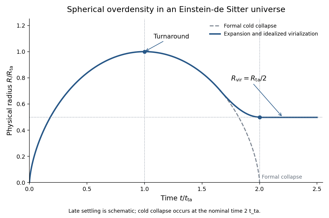
Expansion, turnaround and idealized virialization of a spherical overdensity, compared with formal cold collapse
. Details. 
For a uniform sphere, . At turnaround the coherent kinetic energy vanishes, so . At the final equilibrium, the virial theorem gives , whence . Conservation of energy therefore impliesThis virial radius from turnaround energy assumes conserved mass and energy, negligible surface-pressure/tidal terms, and the same gravitational profile coefficient. The sketch's settling segment is qualitative; the cycloid is the exact pre-virialization cold model, not a dissipative relaxation solution.
To compare with the cosmological density, use in an Einstein-de Sitter universe. The turnaround sphere hasSince the background density falls by four between and , the Einstein-de Sitter virial overdensity isFinally , so assigning the nominal collapse redshift givesThe density ratio eight compares the same object's physical densities at turnaround and virialization; compares its final density with the background at the later collapse epoch.
Follow a conserved mass element from its Lagrangian coordinate to its Eulerian coordinate . The integrated continuity equation giveswhere and the Lagrangian labels are chosen with uniform reference mass per . These equations hold before shell crossing, when the oriented determinant is positive. If are the eigenvalues of , thenFor an irrotational displacement the deformation matrix is symmetric, so these eigenvalues are real. Using the conventional positive collapse eigenvalues , equivalently the eigenvalues of , givesThere is a sign mismatch in the printed pairing of this last expression with eigenvalues of : for the displayed plus-sign displacement map, those eigenvalues give plus signs in the determinant. For example, , makes , so mass conservation gives , not . The corrected eigenvalue convention restores the intended formula without changing the map.
Now take and . The physical trajectory is . Differentiating at fixed givesThe physical derivative in the perturbed direction is . The two transverse directions still have the background acceleration. ThereforeUse the pressureless, background acceleration equation to obtainThis proves the planar exactness of the Zeldovich approximation for the requested full force-divergence equation. The displacement depends on only one coordinate, but the divergence includes all three physical directions; discarding the transverse background terms would give the wrong result. The proof is valid until shell crossing. With the planar gravitational boundary condition fixing the possible spatially uniform force, it is the exact single-stream dust evolution; it does not describe the multistream density by a single invertible map after crossing.
Articles by others on the same topic
There are currently no matching articles.