Plot each observed mortality proportion vertically against its operation count horizontally, retaining the hospital labels. The required points, together with the target and approximate control bands used below, give the following hospital mortality funnel plot.
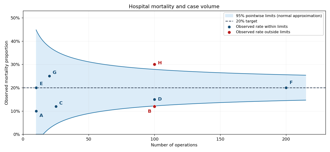
Hospital mortality proportions against operation counts with a 20% target and approximate pointwise 95% binomial control limits
. Details. 
Hospitals sharing an operation count remain separate labeled points; equal observed mortality proportions at different volumes should not be treated as equally precise.
If , the observed binomial proportion has variance . Consequently its standard error is proportional to . A common target therefore produces broad uncertainty at low volume and narrower uncertainty at high volume, forming the funnel-shaped envelope around the horizontal target. The narrowing represents sampling precision, not a predicted change of mortality with volume.
Under the target model , the normal approximation givesThe pointwise 95% binomial funnel control limits are thereforeDraw these curves around the horizontal 20% target, as in the figure. At , the approximate limits are and , so B and H are outside the nominal bands; that is a signal for investigation, not proof of inferior or superior care. The bands use the target variance rather than each hospital's observed rate. They are control limits for possible observations under the target model, not confidence intervals centered on the observed points.
Normal coverage is approximate, especially for the small hospitals; clipping does not repair that approximation. Exact binomial tail limits can be used if exact calibration is needed.
Four advantages of the hospital mortality funnel plot are:
- It presents mortality and case volume together, making the difference in precision between small and large hospitals visible.
- Its volume-dependent control limits distinguish expected sampling scatter from observations deserving investigation, avoiding an indiscriminate ranking of raw rates.
- It displays all hospitals on one interpretable scale with a common target and identifies unusually low as well as unusually high rates.
- It makes the benchmark and statistical assumptions explicit and supports direct comparison as volumes change, without estimating the benchmark from potentially anomalous observations.
It does not automatically adjust for patient severity, referral patterns or data quality, and an outlying point does not establish a causal explanation.
Let indicate a point outside its pointwise 95% limits. Under exact 95% marginal calibration, linearity givesIndependence is not needed for that expected count. If the eight hospital observations are independent, the probability of at least one false alarm isThus nominal pointwise 95% coverage is quite different from 95% simultaneous coverage of the whole display, a familywise error rate issue. Without independence, the product formula need not hold; the union bound is at most .
Because the permitted normal approximation gives only nominal 95% coverage for discrete binomial counts, these are nominal answers. With exact outside probabilities , the exact expected count is and, under independence, the exact probability is .
Three defensible approaches are:
- Use simultaneous calibration, for example Bonferroni correction: give each of eight hospitals outside probability at most . Replace 1.96 by in the normal bands, giving familywise error at most 5% when the marginal tests are calibrated.
- Apply the Holm step-down procedure to valid two-sided binomial p-values. Order them and compare the jth smallest with until the first nonrejection. This controls familywise error while often being less conservative than giving every hospital the same Bonferroni threshold.
- Treat an initial signal as a screen and require prespecified confirmation in independent new data before declaring a persistent deviation, alongside checking case mix and coding. Calibration must include both stages; unrestricted repeated testing until an alarm appears would increase, rather than solve, the problem.
Articles by others on the same topic
There are currently no matching articles.