Work in a meridional plane and denote the interface height by , to distinguish it from an observation coordinate. PutThe interface is , so . Its unit normal into the fluid is proportional to . Consequently the angle between this normal and the vertical satisfiesThe outgoing source P wave has ray direction proportional to , tilting outwards by from the vertical, while the normal tilts inwards. Thus . The tangent addition formula givesDirect substitution simplifies its denominator to and its numerator to . HenceThe denominator is positive, so these are the physical incidence angles in ; the transmitted P wave reaches the fluid rather than propagating back into the solid.
The angles from part (i) have sinesBy Snell law for elastic and acoustic waves, . Both angles lie in , so . The outgoing fluid ray tilts away from the inward-tilted normal by exactly its tilt from vertical; it therefore travels vertically upwards. This is hyperbolic interface collimation of P-waves.
The source-to-interface distance satisfiesOne can verify this by squaring, using . ConsequentlyAdding the vertical fluid travel time from the interface to height givesThus surfaces of equal arrival time in the fluid are horizontal planes. Their leading wave amplitude may vary with : a planar wavefront does not imply a spatially uniform plane-wave solution at every order.
Use local coordinates with the interface , solid below and fluid above, and choose the P-SV displacement potentials convention , . Let the reflected P and SV potential wave amplitudes be , while the transmitted P wave amplitude is . All four waves have the same tangential slownessThe incident and transmitted retarded times have negative , while elastic waves have positive . At the interface all waveform derivatives therefore have the same argument. displacement field continuity givesWith Lamé parameters and , the shear and normal stresses follow directly from differentiation:The fluid has no shear traction, so the coefficient of in must vanish:The coefficient of in the solid stress is ; in the fluid it is . ThusThese are the three required matching conditions; tangential displacement field need not be continuous at a solid–inviscid-fluid boundary.
Put and . From (2), . In (1), the coefficient of simplifies because . Hence . Substitute this into (3) to obtainTherefore the solid-fluid P-wave transmission coefficient isDivision by was only an elimination device; the final expression extends continuously to . The normal-incidence value is . This is a potential coefficient; longitudinal displacement field transmission additionally multiplies it by . The original PDF's bracket lies in the denominator and contains and . The converted TeX misplaces the bracket, substitutes for , and loses the final cosine.
The leading source displacement field isThe second term is one derivative smoother at the leading arrival. At each surface point, use its tangent plane, the angles from (i)–(ii), and the local solid-fluid P-wave transmission coefficient. The incident potential coefficient is , so the transmitted leading potential coefficient isTransport this coefficient along the vertical fluid rays. Their transverse area does not change with height, so ray-tube conservation for a P-wave jump gives no further geometrical spreading. The leading displacement field coefficient is consequentlyThis is the transmitted jump at a collimating solid-fluid interface. Radial derivatives of multiply , and therefore do not contribute to the first derivative jump carried by . A varying transverse wave amplitude does generate smoother later terms, so this construction is a leading-front result, not a complete global plane-wave field.
Since the source is zero before and is there, . Thus displacement field itself does not jump. If exists and is the first nonzero jump, the leading discontinuity is the acceleration jump . More generally, a first jump in gives . The supplied regularity alone does not guarantee a nonzero discontinuity: a source smooth to all orders may have none. The geometrical transfer factor is nevertheless determined.
At , and all three angles vanish. HenceFor large , put and retain , . The relevant limits areWhen , the square-bracket factor in the denominator of is , soThese are signed waveform coefficients; their absolute values give wave amplitude magnitudes. The leading displacement field decays as rather than because grazing incidence adds a small transmission factor to spherical spreading. The leading coefficient is independent of fluid and solid mass densities, although the exact wave amplitude and its higher-order terms depend on them.
The assumptions do not exclude , where and the preceding division is invalid. In this special case exactly, and the square-bracket factor is . Keeping both denominator terms givesIt has no term. This exceptional case matters when requesting an asymptotic formula without an additional restriction on the elastic moduli.
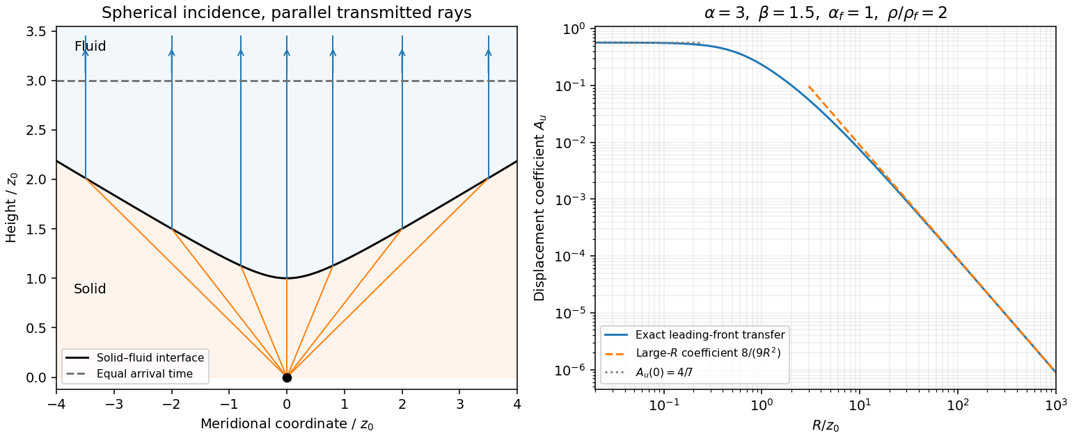
Hyperbolic refraction into vertical rays and the leading transmitted displacement field coefficient compared with its grazing-incidence asymptote
. Details. 
Articles by others on the same topic
There are currently no matching articles.