Choose depth positive downwards and harmonic time dependence . At normal incidence, P waves and the two polarizations of S waves are independent scalar problems: a P wave uses the longitudinal modulus , and an S wave uses the shear modulus . In a uniform layer with wave speed and seismic impedance , write velocity and compressive traction asAt a perfectly bonded interface the velocity and traction are continuous. For incident velocity wave amplitude one from medium 1 into medium 2, these two conditions are and . ThusReflection is determined by seismic impedance, not by speed alone. A step to larger seismic impedance reverses the reflected velocity/displacement field waveform; the pressure reflection coefficient has the opposite sign. Its transmitted pressure coefficient is . Equal seismic impedance eliminates the reflection even when speed and wavelength change. At a free surface traction vanishes and velocity reflects with coefficient ; at a rigid surface velocity reflects with coefficient .
The mean elastic-wave energy flux is for positive real . Therefore the reflected and transmitted energy fractions areA displacement field transmission coefficient greater than one is compatible with conservation of energy; its flux must be weighted by the receiving seismic impedance.
For many layers, use the seismic layer transfer matrix. A layer of thickness has wave phase thickness andThis follows either by eliminating between the two faces or by integrating and . For the complete stack put . With upper and lower half-space impedances , an outgoing lower wave satisfies . Solving this condition gives the input seismic impedanceHere is lower-face velocity divided by upper-face incident velocity, including the propagation wave phase. For lossless layers and real frequency, . This supplies a sensitive check on any spreadsheet or numerical implementation; it is not correct simply to multiply the individual interface transmissions and discard the elastic waves.
The physical reason is repeated wave interference. In one layer between media 0 and 2, let denote the velocity coefficients above and . The first transmitted wave has wave amplitude . Every extra round trip supplies . Summing the geometric series givesIn the time domain the successive arrivals are delayed by , producing reverberation. In the frequency domain the same delayed terms produce resonant maxima and minima. For a layer between identical half-spaces of impedance ,At the layer transmits all the incident energy: the internally elastic waves cancel the direct reflection. Halfway between these resonances, a large impedance contrast gives strong reflection. For unequal exterior impedances, a quarter-wave layer with transforms its lower load to , again giving zero reflection at its design frequency. This matching is narrow-band.
Periodic alternation produces a periodic seismic multilayer stop band. For a cell of two layers with total thickness , the cell matrix has reciprocal eigenvalues , soWhen the absolute value of this expression exceeds one, the infinite periodic medium has no propagating cell mode; a long finite stack has exponentially small transmission. The energy is reflected, not absorbed. Pass bands instead contain oscillatory transmission peaks, becoming more numerous as the stack length increases. Disorder removes the exact cell periodicity but not multiple scattering or frequency-selective interference.
For a concrete reproducible investigation, take , equal one-way travel times in both layer types, exterior impedance , and frequency coordinate . At each layer is a quarter wavelength; one cell has diagonal matrix entries . For cells,It is about for one cell, for four cells and for eight cells. The infinite-cell stop band is . The accompanying calculation also shows the first transmitted arrivals for a single high-impedance slab: their wave amplitudes are at times . Their sum is one, consistent with unit zero-frequency transmission. These calculations illustrate both the spectrum and the pulse train without assuming access to the course's spreadsheet.
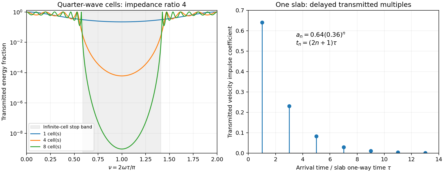
Original transfer-matrix calculations showing a periodic stack stop band and the transmitted reverberation train of one slab
. Details. 
Finally, as for a fixed finite stack, every , so the response approaches that of a direct interface between the exterior half-spaces. Equal exterior impedances give . For wavelengths much longer than a repeating cell, expansion of to first order instead gives an effective medium with averaged mass density and harmonic-mean modulus , where . Its speed is , not generally the arithmetic mean of the layer speeds. Attenuation makes the energy balance an inequality, while for a fixed oblique horizontal slowness the scalar SH calculation uses and . Oblique P-SV waves require coupled displacement field and traction matrices because of mode conversion at a planar elastic interface. Thick evanescent layers require scattering or impedance recursion rather than exponentially ill-conditioned transfer-matrix products.
Work in a meridional plane and denote the interface height by , to distinguish it from an observation coordinate. PutThe interface is , so . Its unit normal into the fluid is proportional to . Consequently the angle between this normal and the vertical satisfiesThe outgoing source P wave has ray direction proportional to , tilting outwards by from the vertical, while the normal tilts inwards. Thus . The tangent addition formula givesDirect substitution simplifies its denominator to and its numerator to . HenceThe denominator is positive, so these are the physical incidence angles in ; the transmitted P wave reaches the fluid rather than propagating back into the solid.
The angles from part (i) have sinesBy Snell law for elastic and acoustic waves, . Both angles lie in , so . The outgoing fluid ray tilts away from the inward-tilted normal by exactly its tilt from vertical; it therefore travels vertically upwards. This is hyperbolic interface collimation of P-waves.
The source-to-interface distance satisfiesOne can verify this by squaring, using . ConsequentlyAdding the vertical fluid travel time from the interface to height givesThus surfaces of equal arrival time in the fluid are horizontal planes. Their leading wave amplitude may vary with : a planar wavefront does not imply a spatially uniform plane-wave solution at every order.
Use local coordinates with the interface , solid below and fluid above, and choose the P-SV displacement potentials convention , . Let the reflected P and SV potential wave amplitudes be , while the transmitted P wave amplitude is . All four waves have the same tangential slownessThe incident and transmitted retarded times have negative , while elastic waves have positive . At the interface all waveform derivatives therefore have the same argument. displacement field continuity givesWith Lamé parameters and , the shear and normal stresses follow directly from differentiation:The fluid has no shear traction, so the coefficient of in must vanish:The coefficient of in the solid stress is ; in the fluid it is . ThusThese are the three required matching conditions; tangential displacement field need not be continuous at a solid–inviscid-fluid boundary.
Put and . From (2), . In (1), the coefficient of simplifies because . Hence . Substitute this into (3) to obtainTherefore the solid-fluid P-wave transmission coefficient isDivision by was only an elimination device; the final expression extends continuously to . The normal-incidence value is . This is a potential coefficient; longitudinal displacement field transmission additionally multiplies it by . The original PDF's bracket lies in the denominator and contains and . The converted TeX misplaces the bracket, substitutes for , and loses the final cosine.
The leading source displacement field isThe second term is one derivative smoother at the leading arrival. At each surface point, use its tangent plane, the angles from (i)–(ii), and the local solid-fluid P-wave transmission coefficient. The incident potential coefficient is , so the transmitted leading potential coefficient isTransport this coefficient along the vertical fluid rays. Their transverse area does not change with height, so ray-tube conservation for a P-wave jump gives no further geometrical spreading. The leading displacement field coefficient is consequentlyThis is the transmitted jump at a collimating solid-fluid interface. Radial derivatives of multiply , and therefore do not contribute to the first derivative jump carried by . A varying transverse wave amplitude does generate smoother later terms, so this construction is a leading-front result, not a complete global plane-wave field.
Since the source is zero before and is there, . Thus displacement field itself does not jump. If exists and is the first nonzero jump, the leading discontinuity is the acceleration jump . More generally, a first jump in gives . The supplied regularity alone does not guarantee a nonzero discontinuity: a source smooth to all orders may have none. The geometrical transfer factor is nevertheless determined.
At , and all three angles vanish. HenceFor large , put and retain , . The relevant limits areWhen , the square-bracket factor in the denominator of is , soThese are signed waveform coefficients; their absolute values give wave amplitude magnitudes. The leading displacement field decays as rather than because grazing incidence adds a small transmission factor to spherical spreading. The leading coefficient is independent of fluid and solid mass densities, although the exact wave amplitude and its higher-order terms depend on them.
The assumptions do not exclude , where and the preceding division is invalid. In this special case exactly, and the square-bracket factor is . Keeping both denominator terms givesIt has no term. This exceptional case matters when requesting an asymptotic formula without an additional restriction on the elastic moduli.
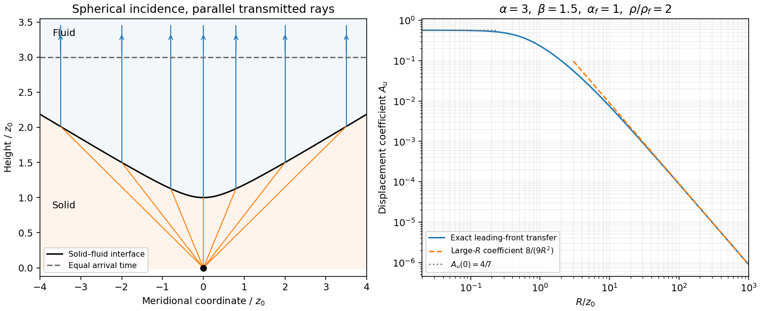
Hyperbolic refraction into vertical rays and the leading transmitted displacement field coefficient compared with its grazing-incidence asymptote
. Details. 
Write , with , and a chosen square root . Squaring givesOne cannot have : the second relation would force , and then the first would require the square of a real number to be negative. ConsequentlyThe bracket has the sign of , proving the causal vertical wavenumber branch equivalenceThis selects the square root analytically in the upper frequency half-plane. At it is ; continuation supplies the outgoing branch for other frequencies. The expression must use this inherited branch rather than an independently chosen square root. For positive real frequency its limit is positive real for a propagating wave and positive imaginary for an evanescent wave.
Let the shear-horizontal wave displacement field be . Its velocity is , and its traction is . The scalar shear-wave equation givesWith and , the first-order velocity–traction system isThese equations remain valid for depth-dependent ; differentiating is essential and one must not incorrectly use when varies.
Where , define the SH input impedance . Differentiating and substituting the two equations gives the SH impedance Riccati equation:The second relation is a one-way scalar equation once the complete SH input impedance is known. It does not discard reflections: describes the actual superposition of both wave directions. At a zero of , may have a pole while the velocity–traction system stays regular.
Use the quadratic spectral flux . For positive real material mass density and shear modulus, differentiation of the velocity–traction system givesBecause is real, . If , then and . This proves complex-frequency SH flux monotonicity:Strictness holds for a nontrivial wavefield: if vanished together at one point, uniqueness of the first-order system would make the entire solution zero. The zero solution is the necessary exception to the literal strict inequality. Across a bonded material boundary , and hence , are continuous; integrating the negative derivative gives strict decrease across any positive-depth interval as well.
Where the SH input impedance is finite, . If , then and all shallower fluxes are larger and positive. They cannot have , since that would make . Thus for every . Likewise, negative real SH input impedance at gives negative flux throughout , excludes velocity zeros there and implies for every .
In a uniform region let on the causal vertical wavenumber branch. The constant Riccati solutions are , and integrating the one-way equation givesSince , the plus solution carries positive downward flux and the minus solution negative upward flux. Writing with , their moduli are proportional to and respectively: each decays in its direction of energy flow.
For complex frequency the displayed quadratic form is the spectral flux diagnostic specified in the question; a genuinely periodic time average is recovered on the real-frequency axis. The decrease here comes from the upper-half-plane convergence parameter, not from material dissipation. At real frequency in a lossless layer the corresponding flux is constant.
Let be either endpoint at which is prescribed, and put , and . Integrating the constant-coefficient velocity–traction system givesTaking the ratio yields the uniform-layer SH impedance update and its accompanying velocity:The initial value sets an arbitrary normalization; specifying impedance alone cannot specify the overall wave wave amplitude. Positive propagates data from , while negative propagates a specified load from , so the same expressions solve both requested initial-value problems.
Expanding sine and cosine givesAbsorbing the reference-point phases into the two constants gives the requested forward/backward exponential superposition. Equivalently, wherever the ratios are defined,The exceptional values give the pure directional solutions. If a denominator in the impedance formula vanishes, propagate the finite pair through that point; this is an impedance-chart pole, not a failure of the physical solution. The upper-half-plane assumptions ensure .
In the lower uniform half-space the causal vertical wavenumber branch has . The downward factor decays as , whereas the upward factor grows there and represents an incoming wave from the lower infinity. The outgoing radiation condition therefore retains only the downward factor and givesFor each uniform layer of thickness , work upwards from its known bottom load . With and , part (iv) givesvelocity and traction are continuous across a bonded interface, so this top impedance becomes the bottom load of the next shallower layer. Repeat up to to obtain . Poles can be handled by carrying or the reciprocal ratio. Since the lower load has positive real part, part (iii) actually ensures that the outgoing whole-stack impedance stays finite with positive real part at all shallower depths in the upper frequency half-plane.
The upper half-space has directional impedance . At , an incident velocity and reflected velocity giveTaking their ratio and solving establishes reflection from a layered SH impedance:Thus no individual deeper reflection coefficients are needed after is known: it contains all underlying interfaces and their coherent multiples. A matched load gives ; the real-frequency limits of zero traction and zero velocity give and . For real frequency and propagating upper and lower half-space waves, the usual energy-flux balance provides a further check on the computed reflection and transmission. A stable implementation for thick layers uses the ratio update or its decaying-exponential version instead of multiplying growing transfer matrices.
Articles by others on the same topic
There are currently no matching articles.