Write for the conformal Hubble parameter and for the velocity divergence of a Fourier mode. Work in the synchronous gauge comoving with the cold dark matter, so . This remains consistent with its pressureless momentum equation . Its density equation then gives .
For the string component, . Thus it makes no contribution to the trace gravitational source in the supplied perfect-fluid model. Substitute and in that trace equation to obtainThe absence of a pressure-gradient term reflects the zero cosmological sound speed of the cold matter.
For the coasting fluid, the continuity and momentum equations becomeThe second equation follows by taking the vector equation; in particular, , which fixes the pressure sign. Differentiate the first equation and use :Eliminating with the cold-matter equation givesThese are equations for the specified idealized barotropic string fluid. A cosmic string network with additional anisotropic stress need not obey the same pressure response.
Separate background stress-energy conservation gives and . ThereforeFor consistency, compute the expansion derivative from the Friedmann equation, rather than assume the printed second hint. Differentiating and using total stress-energy conservation yieldsThe PDF's hint has where is required. It is incompatible with the first hint and conservation, and would not give the requested equation. The expression above is the corrected conformal-time acceleration identity.
For a function , the chain rule givesSubstituting in the cold-matter equation and dividing by producesorThis is cold-matter growth in a matter-coasting-fluid universe; its coefficients depend on the background density ratio, not on .
Multiply the growth equation by :Use the Frobenius method, writing with . The lowest power gives the indicial equationThus the leading powers are and . For , equating the coefficient of givesFor the growing branch , , so and . Taking ,Since , the leading behavior is precisely the usual growing density contrast during matter domination. The negative first correction shows the beginning of suppressed growth as the string fraction increases. The other branch starts as , the familiar decaying matter mode; its exact form is proportional to .
The Jeans length is the physical wavelength at which the restoring pressure term and self-gravity balance. In the elementary static-fluid approximation,Wavelengths longer than are unstable to self-gravitating collapse, whereas shorter ones have restoring sound oscillations. Expansion and relativistic effects modify this elementary criterion. Ideal cold dark matter has , hence no positive pressure-supported Jeans length in these equations. For the specified negative-pressure barotropic string fluid, ; there is no real restoring-pressure Jeans threshold.
For , the matter growth equation has leading termsThe gravitational term is one inverse power smaller than the derivative coefficients. Dropping it at leading order gives , hence a constant mode and a decaying mode. A more controlled check is possible: direct substitution gives as an exact solution. Reduction of order then gives the growing mode, normalized by at early times,The integral grows as , while the prefactor is . Thuswith corrections of order . The perturbation freezes because the matter fraction tends to zero while the coasting fluid controls the expansion.
To describe the requested cold-dark-matter transfer function, its normalization must be specified. The early matter-era Hamiltonian constraint, in the negative-expansion convention for , gives . For the growing comoving dust mode, the continuity equation gives in proper time. Since , this yields . On early superhorizon scales is the conserved curvature amplitude, up to the chosen overall sign, and . This establishes the initial growing behavior rather than assuming identical horizon-entry amplitudes at all epochs. For regular adiabatic modes outside the horizon during early matter domination, , with a -independent constant and primordial curvature amplitude . The matter equation above has no , so at fixed late timeConsequently the density-per-curvature transfer is proportional to on scales entering after equality. The conventional shape transfer, which factors out and the common growth factor, is a plateau, on these scales. Comparing with a matter-only universe that continues growing as instead gives a common amplitude suppression , still independent of . A decline caused solely by later horizon entry would contradict the supplied scale-independent matter equation: the regular synchronous growing solution already evolves outside the Hubble radius. This is the scale-independent matter suppression by a coasting fluid.
There is also a limiting entry scale. Since is constant, define . ThenA mode enters the Hubble radius only if ; enters during matter domination, whereas enters arbitrarily late. Modes never enter in this ideal coasting future. The requested post-equality entrants occupy . The following original diagram distinguishes the two transfer conventions and marks this restricted interval; it does not attempt to model modes entering during radiation domination.
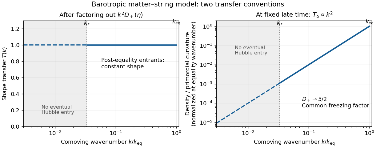
Post-equality cold-matter transfer in the barotropic matter-string model: normalized shape versus density per primordial curvature
. Details. 
The adiabatic initial conditions for separately conserved components have equal . Therefore the radiation relation is replaced here byTo check dynamically, put . At , subtracting two-thirds of the matter equation from the string equation gives . Selecting and no independent relative-velocity mode preserves the relation. Thus the growing adiabatic string density contrast follows the matter mode and is also approximately frozen at late times to leading order in gradients. This is the adiabatic matter-string density relation.
At late times , while and vanish. The homogeneous string equation becomesFor , one solution grows rapidly with exponent approximately , instead of undergoing radiation-like acoustic oscillations. This is a gradient instability of a negative-pressure perfect fluid. For , the growing exponent is only , while the other exponent is approximately . The leading zero-gradient approximation is frozen, but at fixed nonzero superhorizon a slow instability can accumulate over sufficiently long conformal time. The strict gradient limit and infinite-future limit therefore need not commute.
These are the apparent behaviors of the equations given. They do not establish rapid collapse of a realistic cosmic string network: tension, anisotropic stress and the constitutive sound response were excluded in replacing the network by this barotropic perfect fluid. Once the modeled string perturbation becomes nonlinear, the linear calculation itself ceases to apply.
The comoving observer's four-velocity has , so its measured photon energy is , and the comoving momentum is . Let . The null geodesic condition isDivide the temporal geodesic equation by , and use the supplied Christoffel symbols:Differentiating cancels the homogeneous redshift terms. In the remaining first-order term, replace by the unperturbed unit propagation direction :This is the synchronous photon momentum redshift. Background physical momentum decreases as , while the background comoving momentum stays constant.
The spatial geodesic equation gives in the unperturbed universe. Since the temporal equation gives the identical factor for , their ratio is constant at zeroth order. More explicitly, at first order,Every displayed term contains a metric perturbation or its derivative. The orthonormal-frame unit direction differs from by a first-order metric correction, , whose derivative is also first order. Hence , with no background change of direction. Direction corrections multiplied by an already first-order source contribute only at second order.
Express the Collisionless Boltzmann equation in variables and divide the derivative along the photon ray by . Since has no explicit position, direction or conformal-time dependence,This is the chain rule in momentum magnitude and direction. At linear order, , while the last two terms are products of first-order perturbations and can be dropped. The synchronous photon momentum redshift from part i then gives, for spatial Fourier convention ,The factor is essential. It is missing in the PDF's displayed intermediate equation, but follows directly from part i and is needed to obtain its final brightness equation.
Let . Absorbing the common phase-space normalization into , the homogeneous photon energy density is , so the photon brightness perturbation isA small directional temperature change in a Planck distribution gives . Integration by parts yieldsbecause the Planck distribution behaves as at low momentum and decays exponentially at high momentum. Thus . Equivalently, frequency-integrated blackbody radiation energy scales as . Identifying brightness with a single temperature perturbation assumes this blackbody spectral form; the brightness integral itself is defined more generally.
Finally, multiply the corrected transport equation by , integrate and divide by . The spatial streaming factor is independent of , while its gravitational source integrates to . ThereforeThis derives the synchronous photon brightness equation with the normalization and sign fixed, rather than inferring it from the dimensionally inconsistent intermediate formula.
There is first an angular-scale typo in the PDF: smaller angles correspond to larger multipoles, approximately . Small scales relative to the first acoustic peak therefore have , not the printed inequality in the other direction.
The photon-baryon acoustic oscillator produces rapidly varying density and velocity sources around and below the sound horizon. Treating the emission density as a simple long-wavelength gravitational source misses these acoustic peaks and their phases. Silk damping suppresses short-scale perturbations through diffusion before decoupling. The cosmological visibility function has finite width, so different emission times and acoustic phases are averaged rather than sampled on one sharp surface. As tight coupling breaks down, the photon quadrupole and higher moments are generated; Thomson scattering of the quadrupole produces polarization. These require the full photon Boltzmann hierarchy, rather than exactly vanishing emission moments above the dipole. They are the angular-scale limits of instantaneous photon decoupling.
The distinction is important: acoustic evolution and diffusion can already be included in correctly calculated emission and . They do not themselves invalidate collisionless propagation after decoupling. The two-moment, single-time initial condition and omission of scattering after that surface are the approximations used in the requested line-of-sight formula.
For the stated assumptions, multiply the synchronous photon brightness equation by and integrate:Here is the decoupling time. Inverse Fourier transformation shifts each source to the unperturbed rayInsert the initial brightness monopole and Doppler dipole, and divide by four:This is the synchronous Sachs-Wolfe line-of-sight formula. The first term is intrinsic emission temperature, the second is the Doppler effect, and the last is the accumulated gravitational redshift in this gauge. The derivative is the partial conformal-time derivative evaluated on the ray, not its total derivative along the ray. Its integral contains endpoint gravitational effects as well as evolving-potential effects when rewritten in Newtonian gauge; it should not be identified solely with the Integrated Sachs-Wolfe effect.
The direction is photon propagation toward the observer. The observer-to-source sky direction is its negative, so changing that convention also changes the displayed Doppler sign and the ray parametrization. Correct emitter positions and this direction convention are needed to interpret the formula.
Let denote the spatial induced metric and . Its conformally rescaled version has determinant one. The Jacobi determinant derivative formula consequently givesThus the determinant measures the volume-changing part of the spatial metric, while the unit-determinant part contains shape changes. Metric compatibility for the spatial covariant derivative also gives .
There is a sign inconsistency in the PDF. Contracting its defining expression for , with its threading convention and its future normal , givesnot the displayed trace with a minus sign before the divergence. This is the trace of extrinsic curvature with a negative shift. For a concrete check, take , and . The defining formula gives and , whereas the printed trace would give . Reversing the shift convention can produce the other trace formula, but also changes the shift terms in and the normal; the two conventions cannot be combined.
For the requested expansion interpretation, set the shift vector to zero. The sign discrepancy then disappears. A small coordinate volume has proper volume proportional to , and proper time along its normal is . Its expansion rate isThereforeThis is the local volume Hubble parameter, the mean of the three local directional expansion rates. In a homogeneous isotropic background , it reduces to . The interpretation does not require the local expansion to be isotropic: the trace-free part of the extrinsic curvature can still describe shear.
Use and , and define the physical background Hubble parameter by . At first order, the spacetime metric components are , and . Apply the given passive cosmological gauge transformation component by component. The temporal component changes by ; the mixed component changes by ; and the spatial component changes by . HenceThese are the scalar gauge transformations with a background lapse in the paper's sign convention.
Starting in synchronous gauge, preserving both and requiresThe first equation integrates to ; substituting in the second and integrating givesThe arbitrary lower integration limit is absorbed into . Thus specifying synchronous lapse and shift does not fix the origins of the freely falling clocks or all spatial coordinate labels. This is the residual gauge freedom in synchronous gauge.
During cosmic inflation, choosing these clocks remains arbitrary. For example, the mode shifts the spatial potential by and the density perturbation by . In the de Sitter approximation, varies little, so a nearly constant metric perturbation can contain a pure coordinate contribution. An inflaton fluctuation or density contrast in synchronous gauge therefore cannot be declared physical solely from its time behavior. Use a uniform-density curvature perturbation or an appropriate field-based gauge-invariant variable, or fix a physical initial slicing. The exact de Sitter case has no evolving homogeneous density clock, which makes density-defined slicing degenerate.
During the standard hot Big Bang, a cold-matter rest frame supplies a convenient additional condition: imposing zero cold-matter velocity removes the nontrivial spatially varying time-shift mode. Before that condition is imposed, the pure-gauge density contrast for constant is , which decays as in either radiation or matter domination. In conformal time this is proportional to during radiation domination and during matter domination. It can be confused with an independent decaying physical mode unless gauge freedom is fixed. The mode is a time-independent spatial relabeling and must likewise be fixed by a coordinate or initial-metric convention.
Finally, a scalar density transforms by evaluating the homogeneous scalar at the shifted time:To reach Newtonian gauge from synchronous quantities, impose . For the nonhomogeneous scalar modes, chooseUsing background stress-energy conservation, , gives the synchronous-to-Newtonian density transformation with a lapse:The expression includes the lapse factors because dots refer to the arbitrary time coordinate, not automatically to proper time.
Let , and assume so that the density-defined curvature is meaningful. Under the cosmological gauge transformation in part ii,Therefore the two time-shift terms cancel:This is the uniform-density curvature perturbation with the paper's overall sign. On a uniform-density slice it is the spatial curvature potential . Its opposite overall sign is also a common convention, so the sign must be kept consistent rather than imported from another metric convention.
To establish time conservation, write and . Background stress-energy conservation impliesFor constant in the given barotropic equation of state, . Differentiate :Insert both perturbed evolution equations from the hint, keeping the spatial Laplacian :Thus the lapse perturbation and the trace perturbation cancel exactly. The remaining pressure term is the non-adiabatic pressure perturbation . In the assumed barotropic fluid, the perturbed equation of state gives and , so it vanishes. For a Fourier mode,For regular long-wavelength perturbations, the velocity and shear potentials in this combination do not grow as , so the right-hand side is gradient-suppressed when . Therefore is conserved to leading superhorizon order, which is the superhorizon conservation of uniform-density curvature requested.
The statement is not exact for arbitrary finite : the displayed gradient term gives its correction. It also requires adiabatic cosmological perturbations; entropy perturbations in a multicomponent system or a nonbarotropic fluid can give and evolve even at zero gradient order. At exact , and the question's variable is undefined, rather than a well-defined conserved density-slicing perturbation.
Articles by others on the same topic
There are currently no matching articles.