Extend by zero to the negative half-line. Its ordinary Fourier transform is then exactly the Half-range Fourier transform . The Fourier inversion theorem gives the real-line term for ; no endpoint convention at is needed.
It remains to show that each extra contour contributes zero, independently of its coefficient. For , the integral defining is holomorphic. With , multiplication by rotates the sector into , and multiplication by rotates into . Thus the two rotated transforms are holomorphic on their respective upper sectors.
Orient the contours as in the PDF: runs from infinity on the ray into zero and then out along the positive real axis; runs from negative real infinity into zero and then out along the ray. Both have their sector on their left. Smooth decay and integration by parts give in closed lower-half-plane sectors. The factor decays in the upper half-plane for . Close each sector by a large arc; the arc integral vanishes by Jordan lemma, including its short portion near the real axis. The Cauchy integral theorem therefore gives the rotated null contours for half-range Fourier inversion:Adding arbitrary constant multiples of these two zero integrals to ordinary Fourier inversion proves the asserted inversion formula. The constants are arbitrary in this part; selecting them later is what removes an unknown boundary trace.
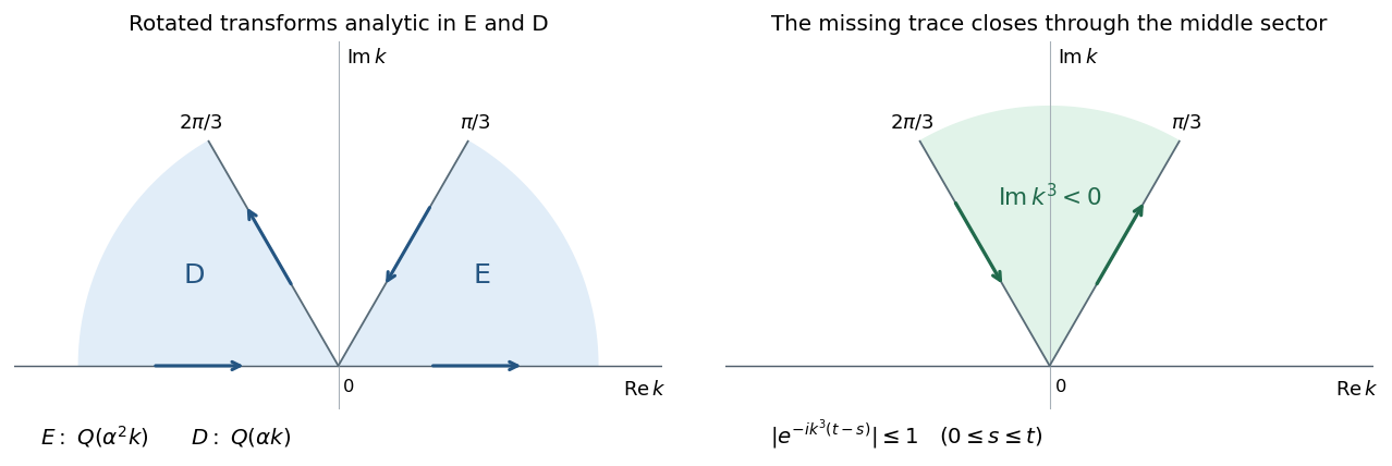
The rotated inversion sectors and the middle sector that eliminates an unknown boundary transform
. Details. 
Define the initial Half-range Fourier transform , and, for each available boundary trace, its finite-time spectral boundary transformTemporarily let also denote the missing trace. Three integrations by parts in giveConsequently the backward-sign Airy half-line global relation isThe spatial transform is holomorphic below the real axis, while each finite-time is an entire function. Moreover, because .
Suppose the missing derivative has order , and put . Its contribution to the right-hand side is , where , , . Apply the inversion from the preceding part at time and selectThe rotated coefficients of that missing trace now equal minus its real-line coefficient. Its entire contribution is thereforeThe real-axis pieces cancel. What remains is the boundary of the middle upper sector, outward on and inward on . In this sector , andis bounded by . The factor decays exponentially throughout the closing arc, overcoming . There are no poles. Thus the Cauchy integral theorem proves the cubic-dispersion elimination of one missing boundary trace and removes every occurrence of the unknown .
For a compact explicit answer, use only the two prescribed traces to form . The three choices areFor each row the solution isAll quantities in this formula are transforms of the given data. On the contour rays is real, so the time exponential is oscillatory; the integrals use the usual limiting interpretation of Fourier inversion. The decay estimate used for elimination belongs to the middle sector, not to or , where can grow.
At , and the preceding inversion recovers . The spectral exponential satisfies the Airy equation with the required minus sign. Differentiating the finite-time amplitudes produces only derivatives of the Dirac delta supported at and zero rotated closed-contour contributions, so the interior equation also holds. Finally, two solutions with the same data have for their difference, so this representation gives zero: each of the three prescribed pairs determines the solution uniquely in the smooth decaying class.
Use the Wirtinger derivative . Since satisfies the Laplace equation, , so is holomorphic. The differential relation is understood as a one-form identity:The differential is needed on its right-hand side. Because this form is closed, its integral is independent of path within the semistrip.
Three spectral primitives are obtained by integrating from the two finite corners and from the infinite end:The last integral is taken horizontally and defines the infinite-end primitive for . Their differences are times the three boundary spectral functions. Using counterclockwise boundary orientation, defineThen , , and . Their sum gives the global relation for .
To express these spectra in boundary data, write , , , , , and . Direct substitution into givesThese are transforms of tangential derivatives of Dirichlet boundary data and the corresponding Neumann boundary data. The outward derivatives are at the bottom, at the top, and at the left.
The boundary spectral representation of a holomorphic function on a semistrip isAll three -rays are oriented outward from zero. To verify the spectral inversion, usewhenever the exponential decays. The positive real ray works for the bottom, the negative real ray for the top, and the positive imaginary ray for the left. Substitution of the boundary spectra therefore turns the boxed formula into by the Cauchy integral formula. This also fixes all orientation signs.
Let denote the Half-range Fourier transforms of , and let denote those of the upward derivatives . Also setIntegrate the tangential derivatives in the three spectral functions by parts. For example, , and . All corner values cancel in . The result is the semistrip Laplace spectral global relation
For , use the sine transformsReality of makes and real, so taking imaginary parts removes the unknown left-side normal derivative. At and the two consequences of the global relation areSubtracting these equations and then substituting back gives the semistrip Dirichlet-to-Neumann sine transforms entirely in terms of the prescribed Dirichlet boundary data:These are the requested transforms of itself. The bottom outward Neumann boundary data have the opposite sign. The apparent division at is handled by a continuous limit whenever the corresponding moments exist; there is no singularity for any .
Let , . Inverting the two orthogonal derivative systems gives, on the vertical axis,and, on the horizontal axis,Using the Wirtinger derivative , these become
Define the appropriate boundary transforms byThe first pair is holomorphic for ; the second pair consists of Half-range Fourier transforms, holomorphic for . Parametrizing the vertical boundary by gives , which must be retained. Substitution yields the quarter-plane oblique boundary spectral functions:Their signs follow from the stated clockwise boundary orientations: upward on the left and inward on the bottom.
Since is harmonic, is holomorphic and the one-form is closed. Closing the physical quadrant at infinity gives the global relationIn this third spectral quadrant the exponential decays on both boundary axes. Set . The relation becomes
All four boundary functions are real. Consequently their transforms obeyand the same identities for . Complex conjugation of the global relation therefore gives its upper-left consequenceIntroduce just one unknown function,It is holomorphic in the upper half-plane. Under the transform-admissible decay assumptions, , so it is bounded there.
For on the positive real ray, use both consequences of the global relation at . Adding them removes and givesFor on the positive imaginary ray, use the upper-left relation and . The resulting single-function spectral elimination for a rational-angle quadrant isBoundary limits from the appropriate transform domains are understood. Every remaining unknown boundary derivative is contained in the one bounded upper-half-plane function .
First resolve the orientation sign in quadrant harmonic spectral inversion. The printed spectral definitions traverse the physical boundary clockwise, whereas both reconstruction rays run outward from zero. Integrating first in gives the kernel . The resulting clockwise Cauchy integral is the negative of the desired holomorphic function. Thus, with exactly the spectral definitions used above, the consistent reconstruction isThe printed plus sign would reconstruct . For a concrete nonzero example, is real, harmonic, smooth on the closed quadrant and decays along both axes. With , it has and . The printed orientation returns the negative of this derivative, so the issue persists even under the stated corner condition.
Let . In the expressions from the preceding part, the coefficient of on the imaginary ray is , and the coefficient on the real ray is . For each of the three allowed sums, . The unknown part is therefore proportional toIndeed, close the first spectral quadrant. For with , , so the large-arc contribution vanishes for bounded . The Cauchy integral theorem proves the equality and eliminates the single unknown function.
Substituting only the known pieces leavesThis already determines the answer from alone. Evaluating the elementary ray kernels gives the more direct rational-angle oblique derivative problem on a quadrant formulaNo denominator vanishes for an interior point of the first quadrant.
There is also a necessary corner compatibility for collinear oblique derivative data. When , the two prescribed derivative directions are opposites, so a continuous corner gradient requires . Together with the stipulated equality, this forces in that case. Existence was assumed, so admissible data must satisfy this additional consequence. Smoothness at the corner and decay at infinity also exclude the homogeneous corner ambiguity in a quadrant Laplace problem; no extra singular or growing term is permitted in the boxed reconstruction.
Articles by others on the same topic
There are currently no matching articles.