Use and . In the interaction picture, fields evolve with the free Hamiltonian, while interactions enter the state evolution through the Dyson series. Write the Klein-Gordon field as , with the positive-frequency part of a quantum field containing annihilation operators and containing creation operators. The mode normalization in the PDF corresponds to and .
The time-ordered product places fields with the latest time on the left. For two bosonic insertions,The normal-ordered product instead moves every creation operator to the left of every annihilation operator, without adding the commutators generated by that rearrangement. Its vacuum expectation value is zero whenever a nonempty set of free-field factors remains.
The mode commutator gives the positive-frequency Wightman functionDefine the Feynman propagator here to be the two-point function itself, rather than that function divided by . ThenEquivalently,The positive-energy pole is below and the negative-energy pole above the real axis. Closing the energy contour integral below for positive time separation and above for negative time separation gives the two terms above. Thus this is the scalar Feynman propagator pole prescription, and . In particular, : the difference between time ordering and normal ordering is the Wick contraction.
For free bosonic fields, the Wick theorem stateswhere runs over all sets of disjoint pairs of indices, including the empty set, and is the set of paired indices. The empty normal-ordered product equals one. This is an operator identity for free fields, understood with smearing or a regulator when products of operator-valued distributions require it.
Here is an inductive proof of the scalar Wick theorem. Sort the arguments chronologically so that is the latest. For any remaining set , commuting the annihilation part of through the creation parts in a normal-ordered product givesThe creation part of is already in the correct position. Every commutator on the right is a scalar, so no further operator rearrangement is needed for it. Because is latest, that commutator is . Assume the Wick theorem for the other fields and multiply its expansion by . The first term of the displayed identity gives every pairing in which index 1 is unpaired; the sum gives every pairing in which 1 is paired with exactly one . Each final partial pairing has exactly one such construction. The one-field identity supplies the base case, proving the theorem by mathematical induction. Applying time ordering restores arbitrary argument order.
Taking the vacuum expectation value retains only complete pairings. Odd free correlators vanish; for example the free scalar four-point function is . These facts explain why propagators are the edges of Feynman diagrams.
For the interacting quartic scalar field theory, the interaction Hamiltonian density is . With a single time ordering acting on external insertions and interaction vertices, the unnormalized numerator expands asApply the proved Wick theorem term by term. Each complete pairing connects external insertions and four-legged vertices by Feynman propagators. There are assignments of four distinct incident legs at a vertex, canceling its factorial. Permuting identical integrated vertices cancels the corresponding part of . Permutations still leaving the labeled graph unchanged give its Feynman-diagram symmetry factor. For example,whereas the two-point tadpole diagram has coefficient , because choosing the two vertex legs contracted with the labeled external fields gives possibilities and the other two contract with each other.
Thus the position-space rules attach to every edge, to every four-legged interaction vertex, and divide by the graph's Feynman-diagram symmetry factor. Fourier transformation gives the momentum-space Feynman rules:Enforce momentum conservation at each vertex, retaining the overall four-momentum delta function. External lines of these correlation functions remain unamputated. The unnormalized expression includes Vacuum Feynman diagrams; dividing by cancels those disconnected vacuum factors. They should not be discarded without that normalization.
There is a time-ordering convention in the printed correlation-function notation worth making explicit. The usual interacting correlator uses the single global time ordering in above. If the displayed is read literally with outside that ordering, the external block and the vertex block are separately time ordered: their cross-contractions are because each external field stands to the left of every vertex field. The same pairing construction then uses for lines within either block and for lines between blocks; in momentum space the latter is . This literal product is different from the conventional globally time-ordered interacting correlator, and does not have the ordinary external Feynman propagators derived above.
The supplied gamma matrices use the mostly-minus metric signature. The Pauli matrix multiplication law gives , hence block multiplication yieldsThe off-diagonal blocks of every connect opposite eigenspaces of this diagonal matrix. Explicitly,Thus , and . The chiral projectors select the upper and lower two-component blocks, respectively.
Write the Dirac spinor as . Substituting the block matrices into the massless Dirac equation gives two independent Weyl spinor equations:They are decoupled because the mass term, which would join the two chirality components, is absent.
For a left-handed plane wave, use . Its coefficient obeysSince , the determinant is . A nonzero coefficient therefore requires the massless mass shell . For positive energy and nonzero , put and parameterize its direction by angles . ThenMultiplication gives and . Hence the left-handed massless plane-wave spinor can be writtenHere is an arbitrary complex normalization; gives . Away from the negative axis one can equivalently takeAt choose instead. These are phase patches for the same one-dimensional kernel. The other frequency branch uses the positive eigenvector for the direction of . At , the algebraic equation vanishes and any two-component coefficient is possible, but no momentum direction or helicity is defined there.
A spatial rotation by about acts on the two-component coefficient by . The negative eigenvector therefore acquires the phase . Since a state with helicity acquires , the positive-energy left-handed particle has . There is only one such spin state at a fixed nonzero momentum, rather than two independent polarizations of the same chiral particle.
The helicity content of a quantized Weyl field also includes an antiparticle with opposite helicity. In the field expansion, the negative-frequency term multiplies an antiparticle fermionic creation operator, while the positive-frequency term multiplies a particle fermionic annihilation operator. Their adjoint roles give conjugate phases for the corresponding created states, so a left-handed field creates particles with and antiparticles with . The right-handed Weyl spinor has the opposite assignments. Quantizing the full massless Dirac field, rather than one chiral component, therefore gives both particle helicities and both antiparticle helicities; every excitation has spin one-half, while chirality determines the helicity of each massless sector.
Keep the printed coupling symbolic and use the Dirac adjoint and . Varying the action with respect to the independent adjoint variable gives the Euler-Lagrange field equationVarying with respect to and integrating its derivative term by parts gives the corresponding left-acting adjoint Dirac equationNow differentiate the axial current . The first equation supplies , and the second supplies . Since and ,Therefore the axial-current divergence for a pseudoscalar Yukawa interaction isBoth the fermion mass and the interaction can break the axial symmetry. This is the classical field-equation identity being asked for, not a claim that quantum composite operators need no renormalization.
There is a convention issue in the original PDF: its interaction is written without an explicit . The Hermiticity of a pseudoscalar Dirac bilinear follows directly fromFor real , the printed interaction is Hermitian if , rather than if is real. The PDF does not specify that is real, so a consistent physical convention is with real . Its interaction is , and the divergence becomes . If were instead required to be real, the printed action would be non-Hermitian; the variational formulas above would still be formal calculations, but the variational adjoint equation would not be its Hermitian-conjugate equation. No missing factor is silently inserted into the solution.
Use the printed interaction, so the Dyson series contributes per vertex before its spinor matrix. The momentum-space Feynman rules areEach interaction vertex has one pseudoscalar line and one incoming and one outgoing fermion-number line. Conserve four-momentum at every vertex, integrate each independent loop momentum with , and divide by any Feynman-diagram symmetry factor. A closed fermion loop contributes an extra minus sign. The external wavefunctions are for incoming fermions, for outgoing fermions, for incoming antifermions and for outgoing antifermions; spinor matrices are multiplied in order along the fermion line. An external pseudoscalar has unit wavefunction factor in standard relativistic normalization. Relative fermionic signs also occur when the external contractions are permuted.
The leading scattering amplitudes are of order . Label the incoming momenta and outgoing momenta , all with positive energy and . Use the Mandelstam variables , and . The tree scattering with pseudoscalar exchange is shown below; dashed edges are pseudoscalar propagators, and arrows indicate fermion-number flow, opposite to the motion of an antifermion.
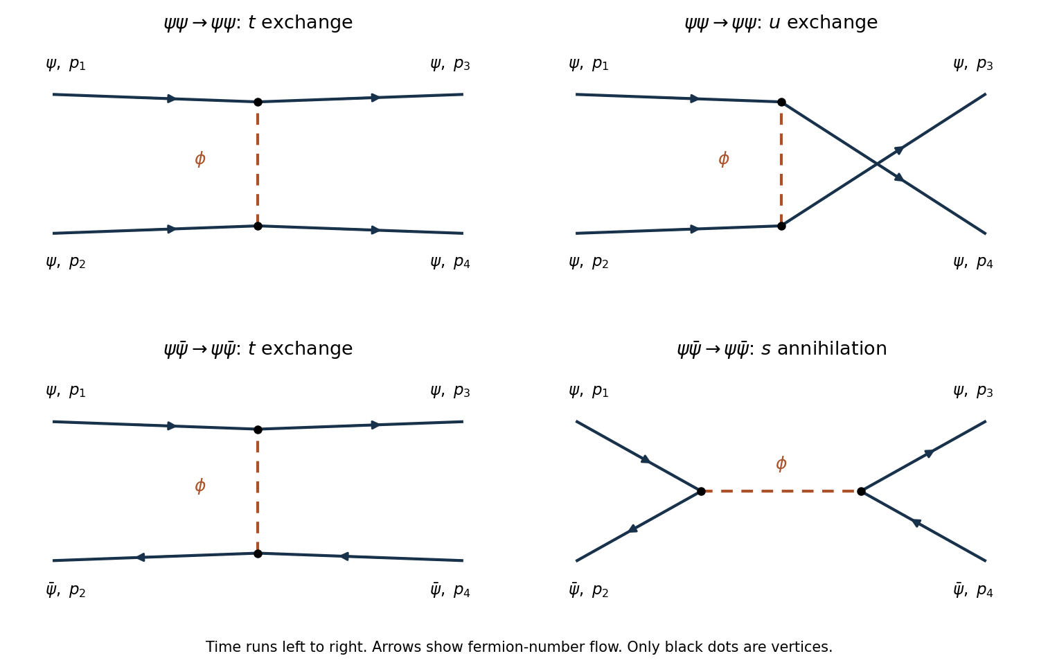
The two pseudoscalar-exchange tree diagrams for fermion–fermion scattering and the exchange and annihilation diagrams for fermion–antifermion scattering
. Details. 
Define the scattering amplitude by . Use standard relativistic normalization for external states and spinors. To fix even the overall signs, suppress the positive state-normalization factors and write the creator order of the two-fermion states as , , and the fermion-antifermion states as , . Spin labels on the are implicit.
For two fermions, the direct graph connects and , while the exchanged graph connects and . The canonical anticommutation relations give signs and for these contractions in the chosen state order. Multiplication of the two vertices and the scalar propagator gives . HenceInterchanging the labels of either pair of identical external fermions reverses this amplitude, as required for the antisymmetric states of fermionic Fock space.
For a fermion and an antifermion, the graphs are exchange and annihilation. Their signs can be derived without guessing an analogy with the first process. The normal-ordered product of the pseudoscalar bilinear contains terms of the formsThe minus in the second term is the antifermion sign of a normal-ordered bilinear. Between the chosen external states, exchange has sign and pair annihilation followed by pair creation has sign . ThereforeChanging an external-state phase can change the common overall sign; it cannot change the relative minus between the two channels. Both amplitudes use the coefficient exactly as printed. For the Hermitian convention discussed in part (a), substitute throughout, or equivalently use vertex from the outset.
Use the free Maxwell Lagrangian in mostly-minus signature. In terms of the spatial electromagnetic four-potential, define and . Thus . Taking the Cartesian components of as coordinates gives the canonical momentaThis sign convention treats here as Cartesian spatial-vector labels; it is not a claim that covariant and contravariant four-vector components coincide.
The temporal momentum vanishes because no occurs. This is the primary momentum constraint of the electromagnetic potential, so one cannot treat all four components as independent unconstrained oscillators. The Legendre transformation for the spatial components gives . After integration by parts, the Hamiltonian isSurface terms vanish for decaying fields or the corresponding regulated boundary conditions. The total constrained Hamiltonian also contains an arbitrary multiplier of . Preserving under time evolution requireswhich is the Gauss law constraint in gauge theory. Both constraints are first-class constraints; they express the gauge invariance , . The electric and magnetic fields are unchanged, so different gauge potentials need not describe different physical states.
One consistent canonical quantization of the electromagnetic field first reduces this redundancy. Choose Coulomb gauge . In the absence of charges, the Gauss law constraint in gauge theory gives ; decay at infinity sets . Residual spatially constant gauge parameters do not change . The remaining variables are the transverse pairs . Their gauge reduction of the Maxwell Hamiltonian isThe two transverse coordinates for each nonzero momentum are the physical degrees of freedom. Treating the constraints as operator identities while retaining unconstrained componentwise commutators would be inconsistent: differentiating would give a nonzero right side even though .
The reduced Dirac bracket, promoted to a canonical commutation relation, instead gives the transverse equal-time commutator:whereIndeed the spatial transverse projector of a vector field is symmetric, has and . Projecting both entries of the unconstrained canonical bracket onto the transverse subspace therefore produces , equivalently the constrained Dirac bracket. The spatial zero mode is excluded by the decay condition; in a finite-volume regulator it must be treated separately.
Choose two orthonormal transverse photon polarization vectors , so thatThe canonical transverse photon field has mode expansionDifferentiate in time to obtain : the annihilation coefficient acquires and the creation coefficient . The oscillator canonical commutation relations areSubstitution into gives times the sum of the two Fourier kernels with phases . The polarization completeness relation and the evenness of make that sum exactly . This derives, rather than presumes, the correspondence between the oscillator and field commutators.
Substitute the mode expansions into . Spatial integration sets paired momenta equal or opposite. The and terms from the electric and magnetic energies cancel because and . The remaining terms are harmonic-oscillator energies. Removing the state-independent zero-point energy by normal ordering givesThe corresponding momentum operator is . These expressions imply and .
Define the Fock vacuum by . Applying creates a photon of energy , momentum , and one of two transverse polarizations. Its mass is zero because . The relativistically normalized state is , with inner product . Smearing these momentum eigenstates gives normalizable wave packets. Repeated commuting bosonic creation operators construct the symmetric multiphoton bosonic Fock space. Circular combinations of the two transverse photon polarization vectors transform with opposite phases under rotations about , giving the two physical helicities .
The same physical states can be obtained while retaining manifest Lorentz covariance through Gupta-Bleuler quantization. Add the Feynman gauge term and quantize four auxiliary oscillator polarizations. Their algebra has an indefinite metric, including a negative-norm temporal excitation. Impose and take the Gupta-Bleuler null-state quotient. Temporal and longitudinal excitations then do not survive as independent physical states. The result agrees with the positive, two-polarization space obtained by Coulomb gauge reduction; covariant gauge fixing is a different implementation of the same physical constraint, not four physical photon states.
Articles by others on the same topic
There are currently no matching articles.