Past exam of the mathematics course of the University of Cambridge / 2012 / iii / Paper 74 / 2

For the elastic filament, apply a variation $\eta (x)$. Two integration by parts operations giveAt a free endpoint both $\eta$ and ${\eta }^{\prime }$ are arbitrary. The free-end bending boundary conditions and the unloaded Euler-Lagrange equation are thereforeHere $A{h}^{\prime \prime }$ is the bending moment and $-A{h}^{(3)}$ the transverse shear-force convention. The equilibrium shapes are affine, reflecting free translation and tilt.

On $L^2(0,L)$ define $K=A{\partial }_x^4$ on $H^4$ functions obeying those endpoints. The self-adjoint endpoint conditions for filament bending annul the boundary formThis proves symmetry. To establish actual self-adjointness, the adjoint-domain boundary form must vanish for every free-end $u$. The endpoint values $u,u^{\prime }$ can be varied independently, forcing $v^{\prime \prime }=v^{(3)}=0$ at both ends. The regular fourth-order expression then gives the same $H^4$ domain for the adjoint. Thus the domains coincide and $K$ is self-adjoint. Also $⟨h,Kh⟩=A\int |h^{\prime \prime }{|}^{2}dx\ge 0$.

A positive-eigenvalue normal mode satisfies $K{W}_n=A{k}_n^4{W}_n$. Solving the constant-coefficient equation gives the sine, cosine, hyperbolic sine and hyperbolic cosine family. To avoid confusing modal coefficients with the filament bending modulus, write those coefficients as $c_1,c_2,c_3,c_4$.

The free conditions at zero require $c_3=c_1$ and $c_4=c_2$. With $q=kL$, the remaining conditions areIts determinant is $2(1-\cos q\cosh q)$. Therefore the free-free bending spectrum isA convenient corresponding eigenfunction iswhere $N_n$ gives unit $L^2$ norm. The stable characteristic equation for free-free bending modes is $\cos q=\mathrm{sech}q$. Intersections or numerical bracketing giveFor the entire positive sequence, let $q_n^0=(n+\frac{1}{2})\pi$. Expanding $\cos q_n$ near its zero and using $\mathrm{sech}{q}_n\sim 2e^{-q_n}$ givesThere are also two zero-energy filament modes, not captured by substituting $k=0$ into the finite-coefficient trigonometric expression. Solving $W^{(4)}=0$ with free endpoints gives the affine kernel. An orthonormal basis of that kernel isThe positive normal modes are orthogonal to both. Including these two rigid-motion modes is essential for completeness; the regular self-adjoint operator on a finite interval has a complete discrete eigenbasis.

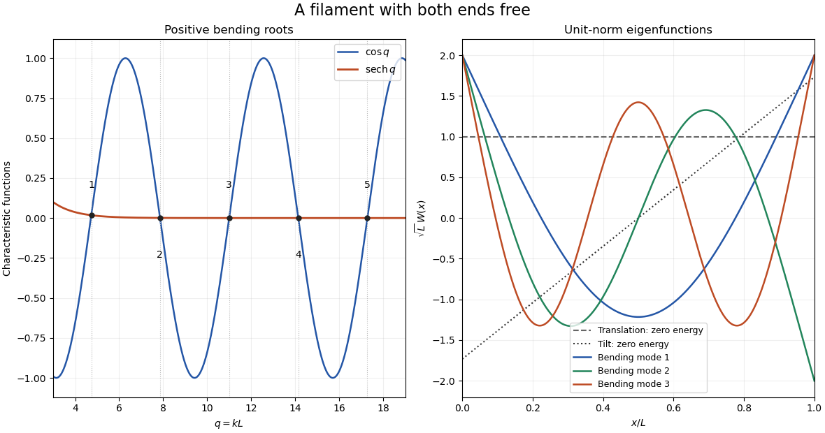
Choose real normalized eigenfunctions, including the two zero-energy filament modes. The expansion isIntegration by parts with the natural endpoints gives $\int W_m^{\prime \prime }{W}_n^{\prime \prime }dx=k_n^4{\delta }_{mn}$. HenceFor each positive mode, the equipartition theorem givesDistinct modal amplitudes are independent centered Gaussian random variables in the canonical bending ensemble.

The rigid translation and tilt amplitudes have no energy cost. Their integrals in the canonical ensemble are unbounded, so a completely free filament has no normalizable equilibrium height distribution and no finite height variance determined by this energy alone. This is a physical qualification of the requested variance, not a reason to omit the bending fluctuations.

Fixing translation and tilt, for example by imposing $\int hdx=\int (x-L/2)hdx=0$, leaves the rigid-motion-projected thermal covariance of a free filament:For unnormalized modes, divide each summand by $\int W_n^{2}dx$. Any prescribed independent variance of the two rigid amplitudes must be added separately; equipartition theorem does not assign it.

The free-filament variance with fixed translation and tilt also has a closed form. Integrate a white noise curvature field twice, and subtract its affine least-squares projection. With $u=x/L$, $t=s/L$, the dimensionless kernel isIt has zero mean and first spatial moment, while its second $u$ derivative is the delta source. Since the covariance is $(k_{B}T/A)\delta (s-s^{\prime })$, integrate its squared kernel to obtainThis conditional profile is symmetric about the midpoint: $P(1-u)=P(u)$, with endpoint value $1/105$ and midpoint value $1/320$. It refers to removing the free rigid motion, not to clamping either end.

The functional derivative is $\delta \mathcal{E}/\delta h=A{h}^{(4)}$, so the overdamped filament bending equation is $\zeta h_t=-A{h}^{(4)}$ with the free-end conditions from (a). Expand the initial shape in the complete orthonormal basis:The overdamped relaxation of a free filament isEach bending mode relaxes on time ${\tau }_n=\zeta /(A{k}_n^4)$; the two zero modes remain constant. Consequently the long-time shape is the affine projection of $H$,The total displacement and its first moment are conserved: integrate $h_t$ and $(x-L/2)h_t$, using $h^{\prime \prime }=h^{(3)}=0$ at the ends. This also checks why the final affine part cannot generally be set to zero. The series defines the $L^2$ solution for arbitrary square-integrable initial data; a classical solution at time zero additionally requires compatible boundary values.