A normal mode, also called an eigenmode, is a pattern of free oscillation in a linear system whose relative displacements stay fixed while a single temporal factor changes their size and sign. For an undamped stable vibrational mode,Here is the mode shape, sets the amplitude, is the eigenfrequency expressed as an angular frequency, and is the oscillation phase. Every snapshot is a scalar multiple of the same mode shape; neighbouring regions may move in opposite directions. Normal modes of a double pendulum show that normal modes also describe coupled discrete systems, beyond strings. Their shapes are eigenvectors, rather than spatial eigenfunctions. [ref]
https://www.feynmanlectures.caltech.edu/I_49.html. Feynman, Leighton and Sands, The Feynman Lectures on Physics, Volume I, Chapter 49
For the ideal wave equation on a string, take a uniform string of length with constant tension and linear mass density . Assume small transverse slope, negligible bending stiffness, no damping, and fixed endpoints. Its wave speed is , and the nonzero normal modes areThe angular frequency is in radians per second; the frequency is in hertz. The wavelength is . The mode shape has loops separated by nodes of a standing wave, including both fixed endpoints. [ref]
As a worked example, choose , , and . Then and , , . Their oscillation periods are , , and . These are deliberately simple model parameters, rather than measurements of a musical instrument. The plot divides displacement by so that the three mode shapes can be compared, and uses each mode's own oscillation period for its snapshots.
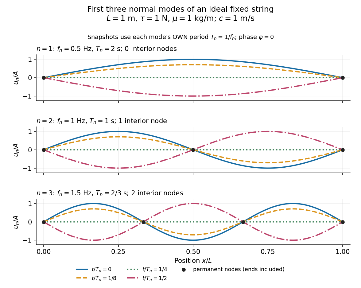
First three ideal fixed-string normal modes at fractions of their own periods; black dots mark permanent nodes
. Details. For , at every point has zero displacement, but most points have nonzero velocity. Only zeros of the mode shape are permanent nodes of a standing wave. At the original mode shape has reversed sign, and at it returns. The synchronized conversion between kinetic energy and potential energy is shown in normal-mode energy exchange.
The short derivation uses separation of variables: substituting into the wave equation gives and . The fixed-end boundary conditions remove the cosine spatial term and require , hence and . Different geometries and boundary conditions give different eigenfunctions; a sine mode shape is a property of this uniform fixed string, not a universal form of an eigenmode.
The usefulness is that a complicated vibration becomes a collection of harmonic oscillators. For sufficiently regular fixed-end initial data, the Fourier sine series givesThe initial displacement and velocity determine and . This is the superposition principle in a Fourier sine basis, and modal energy distribution measures how strongly each normal mode is excited. The striking simplification is that each component keeps its identity while their sum can continually change shape. [ref]
https://www.feynmanlectures.caltech.edu/I_50.html. Feynman, Leighton and Sands, The Feynman Lectures on Physics, Volume I, Section 50-2
These independent normal modes belong to the linear model. At larger slopes, changing tension introduces nonlinear effects and can couple the modes. A linearly damped string still admits a Fourier sine basis, but its temporal factors decay and need not oscillate; its energy dissipation identity for a linearly damped string replaces conservation of energy. More general damping need not leave undamped mode shapes independent.
For two rods of length and mass , one hinged to a fixed point and the other to its free end, use the absolute rod angles from the downward vertical. The small-oscillation mass matrix is and the stiffness matrix is . Their generalized eigenvalue equation gives for . The low-frequency mode has angles of the same sign and the high-frequency mode has opposite signs.
For a finite conservative linear mechanical system with real symmetric positive definite mass matrix and real symmetric stiffness matrix , the normal modes satisfy . Taking the scalar product with and using symmetry in the two equations gives . Distinct-frequency modes are therefore orthogonal in the inner product defined by , even if the dynamical matrix is not symmetric in the ordinary Euclidean inner product. Within a degenerate mode space one can choose an -orthogonal basis.
A pendulum bob and a horizontally moving support of equal mass , with support spring spring constant , have the quadratic potential energy . With , , the normal mode eigenvectors can be normalized to , where . The lower mode is in phase and the upper mode in opposite phase. The positive eigenvalues of the symmetric stiffness-per-mass matrix give the displayed squared angular frequencies.
Three consecutive masses joined by four identical springs of constant between fixed walls have an antisymmetric normal mode with zero central displacement. The two adjacent spring forces cancel on the central mass, while each outer mass experiences restoring force . This proves that the displayed angular frequency is independent of for every positive central mass. The two symmetric modes satisfy and generally do depend on . For , all three mode shapes are , and , with squared frequencies , , .
Two equal masses linked in a line by three identical springs, each stretched to twice its natural length, have longitudinal stiffness matrix and transverse matrix half as large. Equal displacements of both masses select the symmetric modes. Equal longitudinal and transverse release amplitudes produce the title trajectory. It is not closed after one transverse period because the two mode frequencies have irrational ratio . Higher-order geometric terms are neglected in this small-displacement solution.
For a uniform rigid beam of mass and two identical vertical end springs of stiffness , small vertical end displacements have kinetic energy and displacement-dependent potential energy . The mass and stiffness matrices are and . Their generalized eigenvalue problem gives symmetric translation and antisymmetric rocking at the displayed angular frequencies. The centre coordinate contains only the symmetric mode. Neglect spring inertia, damping and finite-angle geometric corrections.
An overtone is an oscillatory mode above the fundamental mode in the same mode family. Waveguide branches are compared at fixed horizontal wavenumber. Their frequencies need not be integer multiples of the fundamental frequency. In a scalar layered guide, additional vertical nodes distinguish successive overtones.
The fundamental mode is the lowest-frequency oscillatory mode for the specified geometry, constraints and, in a propagation problem, horizontal wavenumber. Its frequency need not be a universal constant of the material. In a waveguide it forms the lowest dispersion branch; rigid zero-frequency motions, when present, must be distinguished from oscillations.
For free-end masses joined by two identical springs, the displayed squared frequencies have displacement vectors , and . Distinct eigenvectors are orthogonal in the mass inner product. The zero mode carries translation, while the middle mass does not move in the antisymmetric internal mode. Fixed end springs would give a different spectrum.
An isotropic planar harmonic oscillator of positive charge in a perpendicular magnetic field has two circular normal modes of opposite handedness. With and , the signed angular frequencies have the displayed form for trajectories . A static electric field shifts the equilibrium without changing these frequencies. The clockwise mode has the larger frequency magnitude.
Three identical repelling charges in a one-dimensional harmonic trap have a translation mode , a breathing mode , and a symmetric middle-against-outer mode . Their frequencies are , , and . The translation frequency is unchanged by internal Coulomb forces. Linearizing each pair potential produces a positive spring coefficient .
Changing the trap frequency changes the equilibrium spacing proportionally to without shifting the centre. The old equilibrium displacement from the new one is parallel to the breathing eigenvector. Starting at rest therefore excites that mode alone at linear order; the outer charges oscillate equally and oppositely while the central charge stays fixed.
For a conservative elastic body, the stiffness operator is a self-adjoint operator under compatible boundary conditions. The dynamical operator is self-adjoint in the mass inner product . Choosing mass-normalized normal modes converts the field equation into independent forced oscillators. If the normal modes have mass norm instead, each projected force must be divided by .
For an impulse vector delivered at an unstrained equilibrium, project the velocity jump onto mass-orthogonal normal modes. Multiplying by gives modal velocity coefficient . Its kinetic energy is the displayed expression, including a translational zero mode if one is present. A single endpoint kick in an equal-mass free three-mass spring chain puts fractions into translation and the two internal modes.
Two identical circuits with self-inductance , capacitance and mutual inductance have same-sign and opposite-sign charge modes with . The inductance matrix acts as the mass matrix; positivity requires .
The Hessian of potential energy at a mechanical equilibrium, expressed in specified displacement coordinates. It determines restoring forces to first order. Combining it with the mass matrix gives the dynamical matrix whose eigenvalues are squared mode angular frequencies.
The mass-weighted force-constant matrix for small oscillations. Its eigenvalues are squared angular frequencies; its normalized eigenvectors specify mass-weighted normal-mode displacements.
For diagonal kinetic energy, changes the kinetic quadratic form to . The potential Hessian in these coordinates is .
A breathing mode is a collective normal mode in which a structure expands and contracts radially while preserving its overall symmetry. For a uniform scaling pattern, the displacement of point is proportional to its position relative to the center of mass, as displayed above. In a central spring framework this pattern is a normal mode only when applying the stiffness matrix returns a multiple of the same pattern with the appropriate mass matrix; radial motion alone does not establish an eigenvector.
Three particles are attached to a light taut string between fixed endpoints, with four equal equilibrium segment lengths . The outer two masses are and the central mass is . For small transverse displacement and tension , set . In coordinate order for the two outer particles and the central one, the potential is and the mass matrix is .
The antisymmetric normal mode is with . In a symmetric mode , the equations give and . Their determinant is , whose roots give the displayed symmetric frequencies. Both are positive for positive masses. The physical order of points along the string is ; keeping it separate from the coordinate-vector order prevents a misleading mode sketch.
Consider a straight chain with a fixed wall, spring constants , and consecutive point masses , with the third mass freely ending the chain. Displacements are measured from equilibrium. If the middle mass stays at equilibrium, the two adjacent spring forces must cancel: . The outer equations of motion then reduce to and .
A nonzero oscillatory normal mode with therefore exists exactly when the two outer squared angular frequencies agree, as displayed. Its mode shape is proportional to and its frequency does not depend on . Appropriate initial displacements and velocities confined to this shape keep the middle mass still. For , , , , the common frequency is and the outer displacements are equal and opposite.
Suppose a two-coordinate linear oscillator has independent normal modes as displayed, with positive angular frequencies . For initial displacement and velocity , its solution iswhereThese formulas follow by inverting the two-by-two matrix with columns . Each coefficient evolves by its own scalar harmonic-oscillator equation, and substituting recovers both prescribed vectors. Euclidean orthogonality of the mode shapes is unnecessary; with unequal masses, the natural orthogonality is in the mass inner product of the generalized eigenvalue problem for small oscillations.
Take equal point masses on a massless string, with fixed ends, equal horizontal spacing and constant tension . Small transverse displacements obey , with . The normal modes arewith the displayed positive frequencies. Substitution uses . The endpoint conditions quantize . These are the discrete sine transform modes and form an orthogonal basis, so each initial displacement and velocity decomposes into independent harmonic oscillations. For three masses, convenient relative shapes are , and , with respectively.
Distinct linearly independent normal modes are degenerate if they have the same eigenfrequency. For , their eigenvectors span a common eigenspace; linear combinations in that space are also modes with the same frequency. A symmetry preserving both quadratic energies maps this space into itself. Higher-dimensional irreducible symmetry representations can enforce degeneracy, while perturbations breaking that symmetry can split it. Degeneracies can also occur accidentally without such symmetry protection.
For a large ring of equal pendulums with tangential displacements and nearest-neighbour spring coupling, cyclic translation symmetry gives Fourier modes . The locally straight-chain approximation gives the displayed spectrum. The lowest mode is uniform. For even , the single highest mode alternates signs and has . For odd , perfect alternation cannot close; the highest pair is degenerate and has . For an exact finite regular polygon with straight chord springs, multiply the spring contribution by ; it tends to one in the stated large- limit.
For three equal simple pendulums in a straight open chain with springs only between neighbours, the spring stiffness matrix in displacement coordinates is . Its eigenvectors , and have respective dimensionless eigenvalues . Adding the gravitational restoring term yields the displayed squared eigenfrequencies. These are free spring ends: fixed wall springs would change the matrix and mode shapes.
Releasing the central bob of three identical spring-coupled simple pendulums from displacement excites only the symmetric normal modes. In displacement ratios, . Thus the outer coordinates are and the central coordinate is , where and . The antisymmetric mode is absent by reflection symmetry. The central modulation envelope is , so it never vanishes completely. Slow beats require a small frequency difference; the decomposition itself is exact in the linear model.
Two equal simple pendulums have small horizontal displacements , with their support separation and connecting spring along . If the spring is unstretched at equilibrium, its first-order extension is ; transverse differences change its length only at second order. The quadratic potential is . There is one higher antisymmetric longitudinal normal mode and a three-dimensional eigenspace at : the symmetric longitudinal mode and two independent transverse motions. Pre-tension would lift this transverse degeneracy.
Place equal masses at the six vertices of a regular octahedron and identical unstressed axial springs on its twelve edges. For the invariant axial displacement family , the quadratic potential and kinetic energies areHence . The breathing vector has squared frequency , while every traceless axial vector with has squared frequency . Orthogonal projection onto these subspaces solves any initial condition in this family without an eighteen-dimensional characteristic polynomial.
Two positive masses linked in series between fixed walls by three identical springs of spring constant have equations of motion and . A normal mode exists when , giving the displayed angular frequencies. Its amplitude ratio is : positive for the lower angular frequency, negative for the higher one. Equal masses give amplitude ratios and squared angular frequencies .
The mode shape is the fixed spatial eigenfunction multiplying the temporal factor of a normal mode. It is determined by the governing differential equation and boundary conditions, and may be normalized by a chosen amplitude or energy convention.
Distinct squared traction-free eigenfrequencies in a bounded lossless elastic body have eigenfunctions orthogonal in , by the Betti identity for elastodynamic fields. Normalize one field from each eigenspace. This is an orthonormal set in a separable Hilbert space, so it is countable: disjoint balls of radius less than around its unit vectors must contain distinct points of a countable dense set. Positive and negative frequency partners add at most a factor of two. This argument proves countability without requiring a separate compact-resolvent proof.
An eigenfrequency is the natural frequency associated with a free normal mode. Always specify whether it means the angular frequency or the frequency in hertz. For a uniform fixed-end wave equation on a string, and ; the amplitude does not change either within the linear model. In a generalized eigenvalue problem for small oscillations, the eigenvalue is , rather than itself.
For a first-order system , a real eigenvalue of instead gives a signed eigenfrequency in . A positive imaginary part of gives exponential decay with this sign convention. Thus a complex damped eigenfrequency encodes both oscillation and decay; it is not just the number of cycles per second.
The lowest positive normal mode frequency of an oscillating system is its fundamental frequency. For an ideal uniform string of length with fixed ends and phase speed , . A spatial finite difference approximation has its own lowest positive normal mode frequency, approaching this continuous value as the grid is refined.
For the undamped first normal mode of a fixed string, start at maximum displacement with . In the small-slope wave equation on a string, its kinetic energy and excess potential energy areThe potential energy comes from the extra length under tension: . It depends on slope, so a node of a standing wave need not have zero local potential energy density. These are physical energies, with the mass and tension factors restored to the normalized wave energy. [ref]
https://farside.ph.utexas.edu/teaching/315/Waveshtml/node43.html. Richard Fitzpatrick, Oscillations and Waves, Energy Conservation, equations 6.24-6.29
Integrating and over the string gives in both cases. Using yieldsFor the model , , , and , the angular frequency is , the frequency is , and . The maximum slope is small. At all the energy is potential energy; at the string is straight and all the energy is kinetic energy. At the displacement is reversed and all the energy is again potential energy. The energy curves repeat twice during one displacement cycle, while conservation of energy keeps their sum constant.
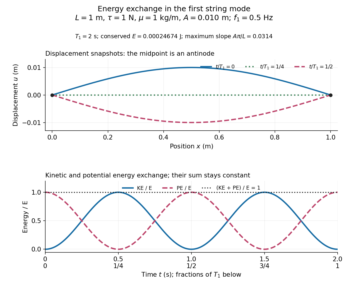
First-mode displacement in metres and kinetic and potential energies divided by the conserved total energy
. Details. A node of an ideal standing wave is a position whose oscillation amplitude is zero: its displacement stays zero for all time. For a nontrivial normal mode , this means . A momentary zero caused by does not make every position a node. In more dimensions the zeros of a mode shape can form curves or surfaces.
For the th normal mode of a uniform fixed-end wave equation on a string, the nodes of a standing wave areThere are nodes of a standing wave including the two endpoints, and interior ones. For and , they lie at , , , and . Each remains stationary through every snapshot in the normal mode diagram; an antinode instead marks a maximum oscillation amplitude. [ref]
A point or surface at which a wavefunction vanishes. In one dimension a simple node of a real stationary wavefunction changes its sign. A node is not generally the same as a classical turning point; for a smooth finite potential, the stationary Schrödinger equation also makes the second derivative vanish at a wavefunction node.
An antinode is a position of maximum oscillation amplitude in a standing wave. For , the antinodes occur atwhere the amplitude is . They sit halfway between consecutive nodes of a standing wave. For the first normal mode, the sole antinode is . It reaches zero displacement at a quarter oscillation period while moving fastest, which illustrates why an antinode is defined by oscillation amplitude rather than instantaneous height.
Articles by others on the same topic



"Normal mode" can refer to different concepts depending on the context in which it is used. Here are a few interpretations: 1. **Physics and Engineering**: In this context, "normal mode" refers to a specific type of oscillation in a system where all parts of the system move in a coordinated way. For example, in mechanical systems, normal modes correspond to the natural frequencies of vibration.