Past exam of the mathematics course of the University of Cambridge / 2013 / iii / Paper 65 / 3

Let $h$ be the water-layer thickness and $z=0$ the horizontal bedrock. In the hydrostatic approximation, with constant ice-interface pressure,The prescribed two-wall stress balance givesIn this subglacial current with constant viscous wall layers, the uniform-pressure ice roof is treated as a movable confining boundary; the closure neglects inertia in comparison with pressure and wall stress. The bulk may be turbulent, while the specified wall viscous boundary layer supplies the linear stress relation. A different turbulent drag law would give a different transport coefficient and similarity exponent.

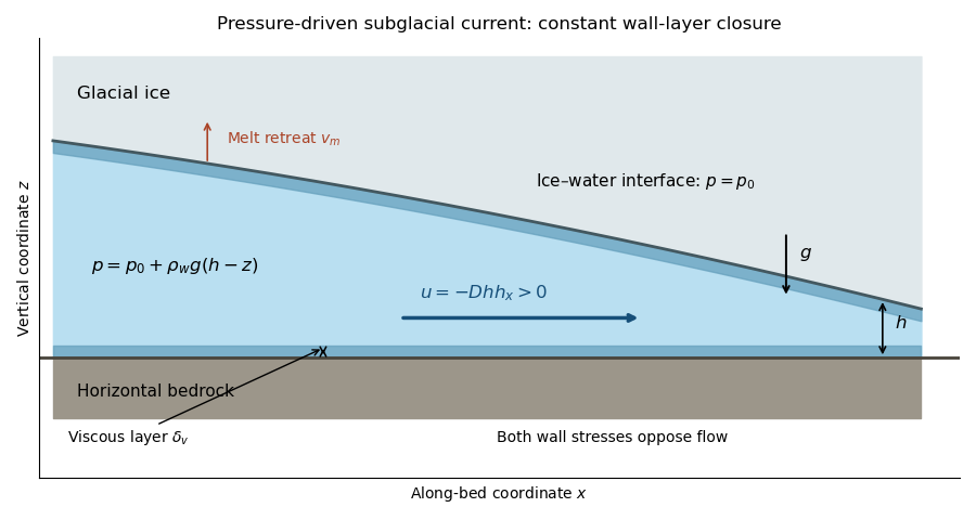
Without melting, the depth-integrated continuity equation gives $h_t+q_x=0$, henceTo write this in the PDF's displayed plus-sign form, its constant must beThe signed value is essential. If the printed $\gamma$ were interpreted as a positive diffusivity, its equation would drive water uphill and be backward parabolic. For example, linearizing around a uniform depth $H$ would give a Fourier perturbation growth rate $+\gamma H^2{k}^2$, whereas the derived physical equation damps it at $-D{H}^2{k}^2$. The plus-sign form is consistent only with the negative $\gamma$ above.

Use the positive transport coefficient $D$ from the preceding solution. The porous medium equation here is $h_t=D(h^2{h}_x{)}_x=(D/3)(h^3{)}_{xx}$. A planar pulse conserves the water cross-sectional area $\mathcal{V}=\int hdx$. If the supplied lake volume is a three-dimensional volume $V$, introduce the constant out-of-plane width $B_y$ and take $\mathcal{V}=V/B_y$; alternatively $V$ may be understood as volume per unit span. A two-dimensional model cannot determine an absolute extent from an unspecified three-dimensional volume alone.

For a symmetric localized release, write $h=t^{-a}f(x/t^b)$. Area conservation requires $a=b$, and balancing the PDE powers gives $a+1=3a+2b$, hence $a=b=1/4$. With $\eta =x/t^{1/4}$, the profile equation isIntegrate once, using symmetry and zero central flux: $D{f}^2{f}^{\prime }=-\eta f/4$. Inside the wet region this gives $f^2=C-{\eta }^2/(4D)$. The dry continuation is zero. Write the result asThe normalization follows from ${\int }_{-L}^{L}hdx=\pi HL/2=\mathcal{V}$. This cubic diffusion pulse has finite support $-L<x<L$, total extent $2L$, and spreading speed $\dot{L}=L/(4t)$. Although $h_x$ is singular at the ideal nose, the flux vanishes there and $u=-Dh{h}_x=x/(4t)$ tends to the finite front speed.

For a one-sided pulse on $0<x<L$ with a reflecting boundary at zero and the same area $\mathcal{V}$, replace $\mathcal{V}$ in the displayed full-line formulas by $2\mathcal{V}$. The power laws are unchanged. These are source-type Barenblatt solutions for an instantaneous localized release; a finite initial lake footprint approaches the profile at long times and may require a virtual time origin, rather than matching this singular initial condition exactly.

Let $K_w$ be the water thermal conductivity, $L_m$ the latent heat of fusion per unit ice mass, and ${\rho }_i$ the ice density. Define $v_m>0$ as the normal ice-retreat speed that enlarges the cavity. With the water thermal boundary layer at $T_s$ on its warm side and $T_m$ at the melting interface, the heat supply per unit interface area is approximatelyThe ice is specified to be uniformly at $T_m$, so no leading sensible-heat flux into colder ice must be subtracted. The Stefan condition is therefore ${\rho }_i{L}_m{v}_m=q_T$, givingEquivalently $K_w={\rho }_w{c}_p{\kappa }_T$ expresses the heat flux in terms of water thermal diffusivity. The imposed temperatures and constant boundary-layer thickness make this melt rate uniform and constant over the wetted interface. Melting adds latent energy demand to the flow; for an isolated finite pulse, maintaining $T_s$ indefinitely would require heat replenishment. The constant-temperature model is consequently an imposed closure, not a prediction of a permanently hot finite water volume.

In the shallow, equal-density approximation, melting supplies water at rate $v_m$ per unit wetted area. Combining this source with the pressure-driven volume flux gives the melting-source gravity-current equation,inside the wet region, with no melting source ahead of the front. In the PDF's signed convention this is $h_t+\gamma (h^2{h}_x{)}_x=v_m$. If ice and water densities are distinguished, the meltwater-volume source is $s_m=({\rho }_i/{\rho }_w)v_m$; the same equations then use $s_m$. Geometrical excavation of ice has rate $v_m$, so a density difference requires the confining ice/water-volume mechanics to be treated consistently. The equal-density shallow model identifies these two volumes.

Let $x_{-}(t)<x_{+}(t)$ bound the current, and $\mathcal{A}(t)={\int }_{x_{-}}^{x_{+}}hdx$ be its volume per span. The moving-boundary integral of continuity isThis exhibits both the melting contribution and any volume swept out by an advancing boundary. For a dry zero-height nose at each end, with no flux through those ends, the boundary terms vanish andwhere the second relation uses constant $s_m$. For a symmetric pulse $\mathcal{L}=2L$, these become $\dot{\mathcal{A}}=2s_{m}L$ and $\ddot{\mathcal{A}}=2s_m\dot{L}$; on a reflecting half-line they are $s_{m}L$ and $s_m\dot{L}$. Multiplication by $B_y$ gives the three-dimensional water volume.

The meltwater production over an advancing footprint can equivalently be expressed as ${\mathcal{A}}_m(t)=s_m{\int }_0^t\mathcal{L}(t^{\prime })d{t}^{\prime }$. At an individual position melting begins only at its wetting time, so new area contributes no finite melt thickness at the instant of arrival. Advancement enlarges the area subsequently melting and hence increases the volume-production rate. The fixed-volume similarity from part (b) cannot simply be reused after adding this source.