Past exam of the mathematics course of the University of Cambridge / 2013 / iii / Paper 65 (Fluid Dynamics of the Environment)

Differentiating the velocity potential gives $u=a\omega e^{kz}\cos (kx-\omega t)$ and $w=a\omega e^{kz}\sin (kx-\omega t)$. Let $A=a{e}^{kz}$ and $\vartheta =kx-\omega t$. To first order in the wave steepness $ka$, evaluate these velocities at the initial parcel position and integrate from time zero:These expressions satisfy both initial conditions and distinguish initial and mean parcel labels in a surface wave. Their actual short-time limits areThe printed expressions omit the integration constants and therefore cannot be the small-time displacement from the prescribed initial point. For example, at $x=0$, they give $Z(0)-z=a{e}^{kz}\ne 0$. This is a genuine inconsistency, rather than a missing step in the calculation.

The intended oscillatory orbit is recovered by using mean parcel coordinates instead. Set $x_c=x+A\sin (kx)$ and $z_c=z-A\cos (kx)$ to this order. ThenThus a deep-water gravity wave produces approximately circular parcel orbits with radius $a{e}^{k{z}_c}$, decaying exponentially with depth. The approximation is one of small amplitude over a wave cycle, not an assertion that these oscillatory coordinates vanish at time zero.

The leading Stokes drift comes from evaluating the oscillatory velocity at the displaced particle position. Taylor expansion givesHere $u_x=-ak\omega e^{kz}\sin \vartheta$ and $u_z=ak\omega e^{kz}\cos \vartheta$. Inserting the initial-position displacements from the preceding solution yieldsIn particular the instantaneous difference is zero at $t=0$, as it must be. The unaveraged constant equality in the PDF is incompatible with its initial labels. Averaging over a period $\mathcal{T}=2\pi /\omega$ removes the oscillatory term:Equivalently, using mean parcel labels and the purely oscillatory displacements gives $a^{2}k\omega e^{2kz}({\sin }^2\vartheta +{\cos }^2\vartheta )$ at this order. This recovers the intended constant result. The period-mean drift is in the wave-propagation direction and decreases as $e^{2kz}$. The corresponding second-order vertical difference is $a^{2}k\omega e^{2kz}\sin (\omega t)$ for initial labels and has zero mean. The resulting horizontal displacement per cycle is $u_s\mathcal{T}$; closed first-order circles do not imply zero second-order transport.

Use the nonrotating linear Boussinesq approximation with reference density ${\rho }_0$ and $N^2=-(g/{\rho }_0)d\bar{\rho }/dz>0$:Let $K_h^2=k^2+l^2>0$, $K^2=K_h^2+m^2$ and $E=e^{i(kx+ly+mz-\omega t)}$. The horizontal momentum equations give $u^{\prime }=k{p}^{\prime }/({\rho }_0\omega )$ and $v^{\prime }=l{p}^{\prime }/({\rho }_0\omega )$. Continuity requires $k{u}^{\prime }+l{v}^{\prime }+m{w}^{\prime }=0$. Thus the internal-wave polarization isPhysical perturbations are the real parts. The density is in temporal quadrature with the vertical velocity, because buoyancy responds to the vertical fluid displacement. Substitution into the vertical momentum equation determines the internal gravity wave dispersion relation,A nontrivial propagating wave requires a nonzero horizontal wave vector and a nonzero frequency. The formulas are not to be divided by $K_h^2=0$: incompressibility excludes a nonzero oscillatory vertical velocity for a purely vertical wave vector.

For the positive-frequency internal gravity wave branch, $\omega =N{K}_h/K$. Differentiating with respect to the components of the wave vector gives the group velocity,The wavefront-normal phase velocity is ${\mathbf{c}}_p=\omega \mathbf{k}/K^2$. Directly,The negative-frequency branch changes both propagation signs but not their orthogonality. Another proof is that $\omega$ is homogeneous of degree zero in the wave vector, so Euler's homogeneous-function identity gives $\mathbf{k}\cdot {\nabla }_{\mathbf{k}}\omega =0$. Energy propagates along constant-phase surfaces, rather than normal to them. When $m=0$, $\omega =N$ and ${\mathbf{c}}_g=0$; the scalar-product result remains true, but there is no nonzero group-velocity direction to describe geometrically.

Use the attenuation coefficient read from the PDF,where here $k$ is the beam wave-number magnitude and the angle convention has $\sin \theta >0$ for the chosen forward attenuation coordinate. The omitted denominator in the TeX is essential both physically and dimensionally. Work in the prescribed along-beam kinematic model, with small parcel excursion compared with ${\lambda }^{-1}$.

The first-order along-beam fluid displacement, initially zero, is $\delta \xi =A\sin (\omega t)/\omega$. Therefore the leading displacement correction to the along-beam velocity isThis oscillatory drift of an attenuated internal-wave beam is oscillatory, soIndeed the scalar parcel equation $\dot{\Xi }=U_0{e}^{-\lambda \Xi }\cos \omega t$ can be integrated exactly:For excursions small enough that the right side stays positive, the parcel returns to its initial along-beam coordinate after each period. This demonstrates the zero net drift in this supplied model. It is not a claim that all components of a viscous beam, or a separately generated Eulerian mean flow, vanish; the question specifies the along-beam component only.

Write $Z=\tilde{z}$ and introduce an arbitrary constant streamfunction scale ${\Psi }_0$, with $\hat{\psi }={\Psi }_0\tilde{\psi }$. The displacement jump condition acquires only a constant prefactor $2{\Psi }_0/\Delta U$, which can be divided out:For the second of the jump conditions for stratified inviscid shear flow, the two derivative terms have common scale $\Delta U{\Psi }_0/h$. Dividing by it givesThe term proportional to the reference density has zero jump by the first condition. ThusNo physical reference-density force has been discarded inside either layer; its continuous interface contribution has canceled. The layer equation becomes ${\tilde{\psi }}_{ZZ}={\alpha }^2\tilde{\psi }$. This explains why only the density anomaly appears in the nondimensional jump condition.

Take $k>0$ without loss of generality, so $\alpha =kh/2>0$, and require decay as $Z\to \pm \infty$. The base velocity is $\tilde{U}=Z$ everywhere; there is no jump in its derivative. Let $C=\tilde{c}$ and $E=e^{-2\alpha }$. A decaying representation that already solves the layer equations isIt is continuous at both interfaces. At $Z=-1$ the value is $A+BE$ and the derivative jump is $-2\alpha A$; at $Z=1$ they are $B+AE$ and $-2\alpha B$. The density anomaly drops by one across each interface. The jump conditions for stratified inviscid shear flow therefore reduce toFor nonreal $C$ the displacement denominators do not vanish. Neutral limiting values are obtained by continuation, rather than by dividing by zero at an interface.

Set $q=J/(2\alpha )$. A nonzero mode requires the determinant to vanish:Expansion gives the dispersion relation for two density interfaces in uniform shear,Uniform shear throughout the exterior is important: replacing it with constant exterior velocities would introduce vorticity jumps and give a different dispersion relation.

For stable density jumps, $J>0$ and $q=J/(2\alpha )>0$. Let $y=C^2$. The two roots of the dispersion relation for two density interfaces in uniform shear areThey are real, and $y_{+}>0$. An exponentially growing normal mode exists precisely when $y_{-}<0$, giving a pair of imaginary phase speeds; the member with positive imaginary part grows in $e^{ik(x-ct)}$ for $k>0$.

Since $y_{+}{y}_{-}=(1-q{)}^2-q^2{E}^2$, this condition is $|1-q|<qE$. Solving both inequalities yieldsAt either endpoint $y_{-}=0$, so the exponential growth rate vanishes. Outside the open band both squared phase speeds are nonnegative and the interfacial modes have real frequencies. This is a modal instability test for the stably stratified configuration; unstable density inversions would require a separate analysis. Within the band the dimensional growth rate is $k\Delta U\sqrt{-y_{-}}/2$.

For large $\alpha$, the evanescent interaction between the two interfaces is proportional to $E=e^{-2\alpha }$. Ignoring it first gives isolated interfacial gravity waves with phase speedsThe lower wave propagating positively relative to its local current and the upper wave propagating negatively have equal laboratory speed whenTheir common speed is zero. This is counterpropagating wave instability: the interfaces communicate through their decaying velocity fields, and near resonance their wave phases can lock while extracting energy from the mean shear.

The instability interval has asymptotic endpoints $J_{\pm }=2\alpha [1\pm E+O(E^2)]$ and widthNear exact resonance the interaction is weak but destabilizing: at $q=1$, $C_{-}^2=2-\sqrt{4+E^2}=-E^2/4+O(E^4)$, so $\mathrm{Im}C\sim E/2$. Thus the resonant band narrows and growth weakens exponentially with separation measured in decay lengths. The resonance here is between two density interfaces in globally uniform shear, not a resonance modified by additional vorticity jumps.

Let $h$ be the water-layer thickness and $z=0$ the horizontal bedrock. In the hydrostatic approximation, with constant ice-interface pressure,The prescribed two-wall stress balance givesIn this subglacial current with constant viscous wall layers, the uniform-pressure ice roof is treated as a movable confining boundary; the closure neglects inertia in comparison with pressure and wall stress. The bulk may be turbulent, while the specified wall viscous boundary layer supplies the linear stress relation. A different turbulent drag law would give a different transport coefficient and similarity exponent.

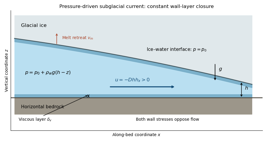
Without melting, the depth-integrated continuity equation gives $h_t+q_x=0$, henceTo write this in the PDF's displayed plus-sign form, its constant must beThe signed value is essential. If the printed $\gamma$ were interpreted as a positive diffusivity, its equation would drive water uphill and be backward parabolic. For example, linearizing around a uniform depth $H$ would give a Fourier perturbation growth rate $+\gamma H^2{k}^2$, whereas the derived physical equation damps it at $-D{H}^2{k}^2$. The plus-sign form is consistent only with the negative $\gamma$ above.

Use the positive transport coefficient $D$ from the preceding solution. The porous medium equation here is $h_t=D(h^2{h}_x{)}_x=(D/3)(h^3{)}_{xx}$. A planar pulse conserves the water cross-sectional area $\mathcal{V}=\int hdx$. If the supplied lake volume is a three-dimensional volume $V$, introduce the constant out-of-plane width $B_y$ and take $\mathcal{V}=V/B_y$; alternatively $V$ may be understood as volume per unit span. A two-dimensional model cannot determine an absolute extent from an unspecified three-dimensional volume alone.

For a symmetric localized release, write $h=t^{-a}f(x/t^b)$. Area conservation requires $a=b$, and balancing the PDE powers gives $a+1=3a+2b$, hence $a=b=1/4$. With $\eta =x/t^{1/4}$, the profile equation isIntegrate once, using symmetry and zero central flux: $D{f}^2{f}^{\prime }=-\eta f/4$. Inside the wet region this gives $f^2=C-{\eta }^2/(4D)$. The dry continuation is zero. Write the result asThe normalization follows from ${\int }_{-L}^{L}hdx=\pi HL/2=\mathcal{V}$. This cubic diffusion pulse has finite support $-L<x<L$, total extent $2L$, and spreading speed $\dot{L}=L/(4t)$. Although $h_x$ is singular at the ideal nose, the flux vanishes there and $u=-Dh{h}_x=x/(4t)$ tends to the finite front speed.

For a one-sided pulse on $0<x<L$ with a reflecting boundary at zero and the same area $\mathcal{V}$, replace $\mathcal{V}$ in the displayed full-line formulas by $2\mathcal{V}$. The power laws are unchanged. These are source-type Barenblatt solutions for an instantaneous localized release; a finite initial lake footprint approaches the profile at long times and may require a virtual time origin, rather than matching this singular initial condition exactly.

Let $K_w$ be the water thermal conductivity, $L_m$ the latent heat of fusion per unit ice mass, and ${\rho }_i$ the ice density. Define $v_m>0$ as the normal ice-retreat speed that enlarges the cavity. With the water thermal boundary layer at $T_s$ on its warm side and $T_m$ at the melting interface, the heat supply per unit interface area is approximatelyThe ice is specified to be uniformly at $T_m$, so no leading sensible-heat flux into colder ice must be subtracted. The Stefan condition is therefore ${\rho }_i{L}_m{v}_m=q_T$, givingEquivalently $K_w={\rho }_w{c}_p{\kappa }_T$ expresses the heat flux in terms of water thermal diffusivity. The imposed temperatures and constant boundary-layer thickness make this melt rate uniform and constant over the wetted interface. Melting adds latent energy demand to the flow; for an isolated finite pulse, maintaining $T_s$ indefinitely would require heat replenishment. The constant-temperature model is consequently an imposed closure, not a prediction of a permanently hot finite water volume.

In the shallow, equal-density approximation, melting supplies water at rate $v_m$ per unit wetted area. Combining this source with the pressure-driven volume flux gives the melting-source gravity-current equation,inside the wet region, with no melting source ahead of the front. In the PDF's signed convention this is $h_t+\gamma (h^2{h}_x{)}_x=v_m$. If ice and water densities are distinguished, the meltwater-volume source is $s_m=({\rho }_i/{\rho }_w)v_m$; the same equations then use $s_m$. Geometrical excavation of ice has rate $v_m$, so a density difference requires the confining ice/water-volume mechanics to be treated consistently. The equal-density shallow model identifies these two volumes.

Let $x_{-}(t)<x_{+}(t)$ bound the current, and $\mathcal{A}(t)={\int }_{x_{-}}^{x_{+}}hdx$ be its volume per span. The moving-boundary integral of continuity isThis exhibits both the melting contribution and any volume swept out by an advancing boundary. For a dry zero-height nose at each end, with no flux through those ends, the boundary terms vanish andwhere the second relation uses constant $s_m$. For a symmetric pulse $\mathcal{L}=2L$, these become $\dot{\mathcal{A}}=2s_{m}L$ and $\ddot{\mathcal{A}}=2s_m\dot{L}$; on a reflecting half-line they are $s_{m}L$ and $s_m\dot{L}$. Multiplication by $B_y$ gives the three-dimensional water volume.

The meltwater production over an advancing footprint can equivalently be expressed as ${\mathcal{A}}_m(t)=s_m{\int }_0^t\mathcal{L}(t^{\prime })d{t}^{\prime }$. At an individual position melting begins only at its wetting time, so new area contributes no finite melt thickness at the instant of arrival. Advancement enlarges the area subsequently melting and hence increases the volume-production rate. The fixed-volume similarity from part (b) cannot simply be reused after adding this source.

Use the planar geometry indicated by the supplied $x,z$ equation and streamfunction; the source heat input is then measured per unit out-of-plane span. Let $\Theta =T-T_0$ and defineThis is the buoyancy part of Darcy law. Let $C_h$ denote the constant heat capacity per volume consistent with the given transport equation; for the fluid heat-flux convention $C_h={\rho }_0{c}_p$. Porosity or matrix heat-storage factors, if retained, must be used consistently in this coefficient and the effective transport parameters.

For plume width $b\ll z$, continuity gives $u\sim wb/z$. Both $u{\Theta }_x$ and $w{\Theta }_z$ are consequently of order $w\Theta /z$: lateral advection must not be discarded. Lateral thermal diffusion is of order $\kappa \Theta /b^2$, while vertical diffusion is smaller by $(b/z{)}^2$. The slender steady porous thermal plume model is thereforeWriting it in conservative form,and integrating across the plume, where $\Theta$ and lateral diffusive/advective heat transport vanish at large $|x|$, provesIn steady state with no lateral heat loss and negligible vertical conductive flux, this equals the heat supplied at the source. Define $Q=\beta F_h/C_h=\int w^{2}dx>0$.

For characteristic velocity $W$ and width $b$, flux conservation gives $W^{2}b\sim Q$ and the advection-diffusion balance gives $W{b}^2\sim \kappa z$. ConsequentlyThe dimensional scales are $b\sim ({\kappa }^2{z}^2/Q{)}^{1/3}$ and $W\sim (Q^2/(\kappa z){)}^{1/3}$. The plume becomes relatively more slender, $b/z\propto z^{-1/3}$, away from the source.

To find the profile, put $\eta =x/b(z)$ and $\psi =-W(z)b(z)f(\eta )$, so $w=W{f}^{\prime }$ andInserting into $u{w}_x+w{w}_z=\kappa w_{xx}$ givesIts coefficient is constant under the derived scaling. Choose the width normalization $W{b}^2=6\kappa z$. Integrating once with decaying velocity derivatives gives $f^{\prime \prime }+2f{f}^{\prime }=0$. A second integration gives $f^{\prime }+f^2=1$ after normalizing the centreline velocity to $W$; symmetry has $f(0)=0$. The decaying, positive solution is $f=\tanh \eta$. Hence the hyperbolic-secant porous plume profile isSince ${\int }_{-\infty }^{\infty }{\mathrm{sech}}^4\eta d\eta =4/3$, the precise amplitudes areThey satisfy both $W{b}^2=6\kappa z$ and $(4/3)W^{2}b=Q$. The derived $u$ supplies lateral entrainment; setting $u=0$ would not reproduce this profile or satisfy continuity.

A heat-weighted head speed of a porous plume estimate follows by filling the column below a head height $Z_h(t)$ with this steady profile. Its excess heat per unit height isConservation of the total injected heat gives $F_{h}t\simeq {\int }_0^{Z_h}\mathcal{H}(z)dz$. Differentiating,Thus a heat-weighted head advances at a speed of order the local centreline velocity and decelerates as $Z_h^{-1/3}$. With $K=(3Q^2/(32\kappa ){)}^{1/3}$,The factor $2/3$ is the energy-conserving estimate for a truncated steady column; the foremost centreline parcels have characteristic speed $W(Z_h)$ instead. The steady calculation does not resolve the transient nose or define an exact sharp temperature front. A truly axisymmetric point-source plume would require different geometry and cannot use this planar profile unchanged.