Past exam of the mathematics course of the University of Cambridge / 2015 / iii / Paper 45 (Statistical Field Theory)

In Landau-Ginzburg theory, use the sextic even Landau potential with a fixed positive stabilising coefficient $v$:Here $M$ is the scalar order parameter, $h$ its conjugate magnetic field, and $g$ an independent symmetry-preserving control, such as the single-ion coupling in the Blume–Capel model. Thus $g$ need not break $M\mapsto -M$, whereas $h$ does. The Blume–Capel mean-field tricritical parameters are one realization; generally, a tricritical point occurs whenTwo controls tune away the quadratic and quartic terms. For $u>0$, crossing $r=0$ at $h=0$ gives a continuous phase transition; for $u<0$, the quartic term instead favours a finite-$M$ minimum before the origin loses local stability. The sextic term bounds the free energy below. The tricritical point joins the continuous and discontinuous transition loci.

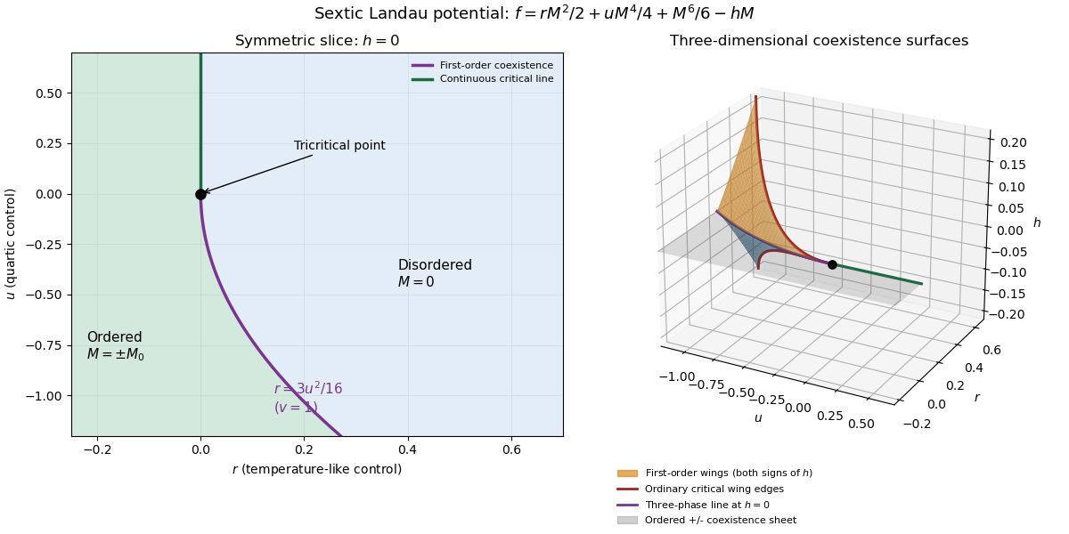
For the symmetric phase diagram, write $s=M^2$. A nonzero stationary point obeys $r+us+v{s}^2=0$. Its free-energy density relative to the origin is $rs/2+u{s}^2/4+v{s}^3/6$. Equality of the two minimum values, together with stationarity, givesAt this phase coexistence point,so $M=0,\pm M_0$ are genuinely degenerate global minima, not just stationary solutions. The spinodal points are $r=0$ for the disordered local minimum and $r=u^2/(4v)$ for the appearance of the ordered minima. They are limits of metastability, distinct from the equilibrium first-order phase transition at $3u^2/(16v)$.

Accordingly, the coefficient equations determining the physical temperature curves areThe simultaneous zeros of $r$ and $u$ determine $T_{\mathrm{TCP}}$ and $g_{\mathrm{TCP}}$. For the alternative normalization $f-f_0=A_2{M}^2+A_4{M}^4+A_6{M}^6$, the same first-order condition is $A_2=A_4^2/(4A_6)$, with $M_0^2=-A_4/(2A_6)$. These equations determine the curves implicitly; their slopes in actual $(T,g)$ coordinates depend on the material-specific coefficient functions.

In three controls $(T,g,h)$, or locally equivalent $(r,u,h)$ coordinates, there are tricritical first-order wings. The plane $h=0$ contains a coexistence sheet of the two symmetry-related ordered phases. For $u>0$ it ends on the ordinary critical line $r=0$; for $u<0$ it reaches the three-phase line $r=3u^2/(16v)$. Two further first-order surfaces extend from that line into $h>0$ and $h<0$. Across a wing, two minima of the same sign but different magnitudes exchange global stability; the field favours that sign. Each wing ends on an ordinary critical edge where those minima and their intervening maximum merge. The three surfaces and their critical boundaries meet at the tricritical point.

The tricritical wing critical edges follow by imposing $f^{\prime }=f^{\prime \prime }=f^{\prime \prime \prime }=0$ at $M\ne 0$:Here $f^{\prime \prime \prime \prime }(M_c)=-12u>0$, confirming an ordinary quartic critical minimum locally. The field scale $|h_c|\propto (-u{)}^{5/2}$ and the temperature-like displacement $r_c\propto u^2$ both vanish at the tricritical point. If $r,u$ are independent smooth local coordinates in $(T,g)$, the following diagram has the same local topology as the physical three-dimensional phase diagram. Its surfaces use exact equal-minimum conditions, as described by tricritical wing coexistence factorization.

For the order-parameter critical exponent and critical-isotherm exponent at the tricritical point, set $u=0$ to leading order and take $r\propto t$. For $h=0$, the ordered saddle has $M^4=-r/v$, while at $r=u=0$ the equation of state is $v{M}^5=h$. Hence the tricritical mean-field critical exponents areThese are mean-field critical exponents. Below the tricritical upper critical dimension they need not be the interacting exponents, and at that dimension logarithmic corrections can accompany the powers. Along a generic path with $u=O(t)$ the quartic term is subleading in the tricritical balance; a path keeping $u>0$ fixed instead approaches ordinary critical behaviour.

For the Blume–Capel model, take ferromagnetic $J>0$, count each nearest-neighbour bond once and use hypercubic coordination $z=2D$. The nearest-neighbour direction sum in the printed Hamiltonian is understood implicitly. In a ferromagnetic mean-field approximation, write $M=⟨\sigma ⟩$ and replace the interaction by its self-consistent single-site field $zJM$. The single-site partition function and variational free-energy density areThe first term prevents double counting the interaction energy. Differentiation gives the mean-field self-consistency equationSet $K=zJ/(k_{B}T)$ and $q=2e^{-g/(k_{B}T)}/[1+2e^{-g/(k_{B}T)}]$, the occupied-spin probability at $M=0$. Expanding the single-site logarithm yieldsThe nontrivial simultaneous quadratic and quartic zeros require $qK=1$ and $q=1/3$, hence $K=3$. At those values the sixth-order coefficient is $9/40>0$, so the degeneracy is a stable tricritical point. The mean-field tricritical parameters areThis is a mean-field result, not a dimension-independent exact lattice transition temperature. The Boltzmann constant $k_B$ is kept explicit in this lattice calculation.

For the Gaussian critical exponents, use dimensionless statistical-action conventions, with the Boltzmann factor $e^{-H}$. If $H$ is an energy, apply the following to $H/(k_{B}T)$ and absorb that smooth factor into the couplings. Choose the Fourier transform conventionReality gives $\tilde{\varphi }(-p)=\tilde{\varphi }(p{)}^{\ast }$. The Fourier-space statistical Hamiltonian isThe source term is not multiplied by one half. Completing the Gaussian functional integral gives $⟨\tilde{\varphi }(p)⟩=\tilde{J}(p)/({\kappa }^{-1}{p}^2+m^2)$ and the connected Fourier-space two-point correlation functionAssume $m^2>0$ for the stable massive Gaussian field theory. In the continuum long-distance theory, the real-space correlation function is the Green kernel of $-{\kappa }^{-1}{\nabla }^2+m^2$. Away from its source, a radial ansatz $G(R)\sim R^{-(D-1)/2}{e}^{-R/\xi }$ gives, at large $R$, $m^2-{\kappa }^{-1}{\xi }^{-2}=0$. Equivalently the propagator pole is at $p^2=-\kappa m^2$. Thus the exponential correlation length isAt $m=0$ the correlation length diverges. A sharp momentum regulator itself introduces artificial oscillatory long-distance tails; this length describes the physical continuum pole or a local/smoothly regulated model on distances large compared with $a$.

For a momentum-shell renormalization group step with $b>1$, split the Fourier modes into retained modes $|p|<\Lambda /b$ and eliminated modes $\Lambda /b<|p|<\Lambda$. Define ${\tilde{\varphi }}_B(p)$ as the retained field. Integrating the eliminated modes is exact for a Gaussian field theory; a uniform source acts only on the zero mode, so this integration produces a field-independent free-energy term. Rescale $q=bp$ and set ${\tilde{\varphi }}_B(p)=\tilde{Z}{\tilde{\varphi }}^{\prime }(q)$. The retained quadratic action becomesKeeping the gradient coefficient fixed requires $b^{-D-2}{\tilde{Z}}^2=1$. For $J=h$, the source term is $-h{\tilde{\varphi }}_B(0)$, so the complete Gaussian rescaling isThe corresponding real-space field obeys ${\varphi }_B(x)=b^{(2-D)/2}{\varphi }^{\prime }(x/b)$; confusing that real-space factor with $\tilde{Z}$ would change the source exponent incorrectly.

Let $F$ be free energy per original volume, with $t$ proportional to $m^2$. Rescaled volume is $V^{\prime }=V/b^D$, so the Gaussian free-energy scaling relation isA field-normalisation Jacobian can be included in the field-independent shell term. For any finite step on positive-mass modes, that background is analytic near $t=0$. Subtract regular backgrounds and choose $b=t^{-1/2}$ on the massive side. The usual homogeneous singular scaling then givesThese are Gaussian critical exponents for the stipulated Gaussian approximation. A useful check is its source-dependent contribution $-h^2/(2m^2)$: $D/2-2\Delta =-1$ gives precisely that power of $t$.

There is a qualification to a strictly pure-power singular free energy. The Gaussian free-energy logarithm at effective dimension two in $D=2$ contains $t\log t$ after subtracting analytic terms. Thus the displayed exponent assignments remain the formal power indices, but at $D=2$ the advertised homogeneous expression needs this additive logarithmic term. A purely quadratic theory also cannot stabilise the ordered $t<0$ phase or the zero-mass zero mode at nonzero $h$; the scaling calculation is taken from $t>0$, and an ordered-phase continuation requires stabilising interactions.

At a uniaxial Lifshitz point, the quadratic kernel instead isThe vanishing coefficient of $p_{\parallel }^2$ is an additional tuning that distinguishes this Lifshitz point from an ordinary critical point. Use a factorised cutoff, retain $|p_{\perp }|<{\Lambda }_{\perp }/b$ and $|p_{\parallel }|<{\Lambda }_{\parallel }/c$, and integrate its complement. A rectangular or cylindrical retained region is suitable; its precise boundary is not an exponent. This is a uniaxial Lifshitz Gaussian renormalization step.

Set $q_{\perp }=b{p}_{\perp }$, $q_{\parallel }=c{p}_{\parallel }$, and ${\tilde{\varphi }}_B=\tilde{Z}{\tilde{\varphi }}^{\prime }$. The momentum measure acquires $b^{-(D-1)}{c}^{-1}$. Keeping both kinetic coefficients fixed requiresTherefore the anisotropic blocking and source factors areThe anisotropic effective dimension is $d_{\mathrm{eff}}=D-1+1/2=D-1/2$: one parallel coordinate contributes half the scaling weight of a perpendicular coordinate. The rescaled-volume factor is $b^{-d_{\mathrm{eff}}}$, soChoosing $b=t^{-1/2}$ gives the requested Lifshitz Gaussian exponents:Again $(D-1/2)/2-2\Delta =-1$, checking the uniform-source susceptibility. The associated length powers are ${\xi }_{\perp }\sim t^{-1/2}$ and ${\xi }_{\parallel }\sim t^{-1/4}$. A Gaussian determinant has the analogous logarithmic exception if its effective dimension equals 2. Interactions can alter these exponents; dimensional rescaling here solves the specified Gaussian model.

In the convention implied by the printed expansion, the truncated two-point quantity is the inverse connected propagator, or one-particle-irreducible two-point vertex:It is the second functional derivative of the quantum effective action (or statistical Legendre effective action) about a translationally invariant zero-field equilibrium. The relation follows from the inverse Hessian relation for a connected two-point function. The subscript $c$ in $G$ already removes disconnected one-point products; the word “truncated” here is not a request to subtract that product a second time. Nor is a general amputated connected correlation function interchangeable with a one-particle-irreducible correlation function.

Use the zero-momentum renormalized mass $R=m^2(0,T)$ in the free propagator ${\tilde{G}}_0(p)=(p^2+R{)}^{-1}$, and split the quadratic coupling into $R$ plus a mass counterterm $\delta m^2=m^2(\Lambda ,T)-R$. The self-energy $\Sigma (p)$ is the sum of loop 1PI insertions, excluding the separately displayed counterterm. Summing repeated insertions by Dyson resummation givesThe sign convention is that a positive tadpole shifts the inverse propagator upwards. At first order, the connected correlation function correction is $-G_0^2\Sigma$, consistent with this inverse-propagator convention. A different split between the reference mass and counterterm produces the same renormalized result.

For the positive quartic interaction $g{\varphi }^4/4!$, the one-loop tadpole diagram has no external-momentum dependence. Its symmetry factor is $1/2$: assigning the two external legs to four vertex fields gives $4\cdot 3$ contractions, and division by $4!$ gives $1/2$. With the dimensionless statistical-action convention,The physical zero-momentum condition $\tilde{\Gamma }(0)=R$ sets $\delta m^2+{\Sigma }_1(0)=0$, hence the one-loop mass relation isWriting the internal line with $R$ is a renormalized or self-consistent one-loop convention. Away from critical infrared singularities it differs from a bare-mass insertion only at higher perturbative order. This equation does not by itself provide exact critical exponents once loop corrections become large.

For $D>2$, subtract the critical-temperature condition $0=m^2(\Lambda ,T_C)+(g/2)I_D(0)$. Take $g$ and the regular coefficients at their critical values, absorbing smooth changes into a coefficient $A>0$. Sincethe one-loop critical-mass subtraction becomesLet $K_D$ be the area of the unit $(D-1)$-sphere divided by $(2\pi {)}^D$. Radial integration gives $J_D(R)=K_D{\int }_0^{\Lambda }{k}^{D-3}(k^2+R{)}^{-1}dk$.

For $D>4$, $J_D(0)=K_D{\Lambda }^{D-4}/(D-4)$ is infrared finite, so it merely renormalises the coefficient and $R\propto T-T_C$ is consistent. For $2<D<4$, setting $k=\sqrt{R}x$ yieldswith a finite positive dimensionless integral. The correction is singular relative to the term $R$, invalidating the finite-coefficient linear-mass assumption. At $D=4$,so the boundary is logarithmically marginal. For $D\le 2$, even the subtraction using $I_D(0)$ needs an infrared regulator; it cannot be used to restore a finite linear critical expansion. Thus the ordinary upper critical dimension isA fixed-coupling self-consistent one-loop formula is not the full marginal renormalization group analysis, but its logarithm already shows why an uncorrected linear power law is not generic at $D=4$.

At a tricritical point, both the quadratic and quartic scaling directions must be tuned; the leading stabilising interaction is sextic. With canonical scalar-field engineering dimension $(D-2)/2$, the sextic coupling has eigenvalue $D-6(D-2)/2=6-2D$. It becomes marginal at $D=3$, givingLower even couplings generated by coarse-graining must remain tuned. This is why using an untuned quartic tadpole to diagnose a tricritical point would give the wrong boundary. The tricritical sextic beta function supplies marginal logarithmic corrections at three dimensions.

For a general multicritical even Landau potential, assume the lower stabilising even terms have been tuned away and the first remaining one is $A_{2n}{M}^{2n}$, with $n\ge 2$ and $A_{2n}>0$. Minimising the potential on its ordered branch givesIts curvature at the minimum is $4(n-1)a_2|t|$. For a finite positive gradient stiffness $c$, the longitudinal correlation length therefore scales as $\xi \propto |t{|}^{-1/2}$. The Ginzburg criterion compares the order-parameter fluctuation averaged over a correlation volume with this squared mean-field value. Keeping momenta of order ${\xi }^{-1}$ or less,Consequently the multicritical Ginzburg ratio behaves asOnly for a positive exponent do these relative fluctuations vanish on approaching the critical point. Thus the general upper critical dimension isEquivalently the interaction eigenvalue $y_{2n}=2n-(n-1)D$ vanishes there. The cases $n=2$ and $n=3$ reproduce 4 and 3 respectively.

For $D<D_C$, the ratio diverges and the mean-field assumptions lose self-consistency arbitrarily close to the transition. At $D=D_C$ the marginal Ginzburg criterion is scale-independent at this leading estimate, rather than tending to zero; the criterion alone does not prove a divergence or force new power indices. Marginal interactions require a renormalization group calculation and generally give logarithmic corrections, as for the quartic and sextic cases above. The boundary case is marginal, not a strict power-law divergence. This qualifies the printed wording at equality while recovering the requested upper critical dimensions.