Past exam of the mathematics course of the University of Cambridge / 2015 / iii / Paper 80 (Complex and Biological Fluids)

Use the Cartesian streamfunction convention $u_x={\partial }_y\Psi$, $u_y=-{\partial }_x\Psi$. In the creeping-flow regime implicit in the question's biharmonic equation hint, the Stokes equations are $\mu {\nabla }^2\mathbf{u}=\nabla p$, $\nabla \cdot \mathbf{u}=0$. Taking their curl eliminates pressure and givesThe fluid occupies the region above the actual sheet; the perturbation calculation expands its boundary about $y=0$. In the swimming frame the material velocity is $(0,-\omega y_0\cos (kx-\omega t))$. The vertical kinematic condition and the supplied Navier slip boundary condition therefore give, at $y=y_0\sin (kx-\omega t)$,At infinity, ${\Psi }_y\to U$ and ${\Psi }_x\to 0$, with bounded velocity and no imposed shear; all fields are periodic in $x$ with period $2\pi /k$. The sign is important: a sheet translating at $-U{\mathbf{e}}_x$ sees the remote fluid translating at $+U{\mathbf{e}}_x$.

Set $X=kx$, $Y=ky$, $\tau =\omega t$, $\psi =k^2\Psi /\omega$, and $U^{\ast }=kU/\omega$. The two dimensionless parameters are the small-slope approximation parameter $ϵ=k{y}_0$ and dimensionless slip length $\delta =k\gamma$. With $\theta =X-\tau$, the dimensionless biharmonic stream function for planar Stokes flow satisfiesExpand $\psi =ϵ{\psi }_1+{ϵ}^2{\psi }_2+\cdots$ and $U^{\ast }=ϵU_1+{ϵ}^2{U}_2+\cdots$. At first order,The decaying first harmonic of the biharmonic equation has the form $(A+BY)e^{-Y}\sin \theta$. The vertical condition fixes $A=1$ and excludes a cosine component. The horizontal condition givesThus $(1+2\delta )(B-1)=0$ and $B=1$ for every $\delta \ge 0$. The spatially averaged first-order streamfunction is affine in $Y$; its Navier slip boundary condition forces $U_1=0$. ThereforeThis first-order slip independence of a transverse sheet is independent of slip length. Its surface tangential velocity and surface shear are both zero: $({\psi }_1{)}_Y(0)=0$ and $({\psi }_1{)}_{YY}(0)-({\psi }_1{)}_{XX}(0)=0$. This explains why the first-order streamfunction agrees with the no-slip boundary condition.

To find the slip-enhanced swimming speed of a transverse sheet, expand only the Navier slip boundary condition through second order. Put $Q_j=({\psi }_j{)}_{YY}-({\psi }_j{)}_{XX}$. Taylor expansion at the displaced boundary yieldsDirect differentiation givesHenceAverage over $X$. The zero Fourier series mode of a biharmonic streamfunction is a cubic polynomial in $Y$; bounded velocity at infinity removes the quadratic and cubic terms. Thus its velocity is the constant $U_2$, and its averaged shear $⟨Q_2{⟩}_X$ is zero. The mean boundary velocity determines Taylor-sheet swimming speed principle then givesThe even remainder follows because changing the sign of the amplitude is equivalent to a half-period phase shift. In dimensional form,For the Navier-slip Taylor swimming sheet, the ratio of speed to the no-slip value is $1+2\delta >1$ whenever $\delta >0$: slip increases the swimming speed. The expansion is for fixed $\delta$ as $ϵ\to 0$; it is not a uniform prediction of arbitrarily large speed if the slip length is allowed to diverge with the inverse amplitude.

Let $s$ be arclength, $\mathbf{t}={\partial }_s\mathbf{r}$ the unit tangent, and $\mathbf{v}$ the local filament velocity relative to the fluid. The resistive-force theory force per unit arclength, exerted by the fluid on the filament, isThe parallel and perpendicular drag coefficients of a slender filament are proportional to dynamic viscosity. For radius $a$ and a relevant axial cutoff length $\ell \gg a$, the anisotropic slender-filament drag from Stokeslet integration gives the leading logarithmic formsThe cutoff may be set by filament length or deformation wavelength. End shape and the choice of cutoff change order-one constants inside the logarithms. Slender-body theory also includes nonlocal interactions that the local resistive-force theory approximation omits. Typically ${\xi }_{\perp }>{\xi }_{\parallel }$, with ratio tending to two in the slender limit; this drag anisotropy enables propulsion.

Write $C={\xi }_{\perp }-{\xi }_{\parallel }>0$. For a small-amplitude planar deformation, $\mathbf{t}=(1,y_x)+O(y_x^2)$ and the leading transverse velocity is $y_t$. Exact inextensibility requires the quadratic longitudinal displacement of an inextensible planar filament: if $X(s,t)=s+X_2(s,t)$ and $Y(s,t)=y(s,t)$, then $X_{2,s}=-y_s^2/2$ to this order. Its velocity is quadratic and has zero time average for a periodic material cycle without mean axial drift. Thus the fixed material abscissa in the question is leading-order notation; this correction does not change the averaged propulsive term below. An imposed mean translation would contribute its separate ordinary axial drag.

To leading nonzero order,The time-averaged deformation-induced propulsive force of a periodic planar filament and power of a periodic planar filament are consequentlyThese are the leading quadratic functionals. Their signs refer to force on the filament. For example, $y=a\sin (kx-\Omega t)$ gives negative $F_x$, opposing the direction of wave propagation.

Let $\eta (x,t)$ be an arbitrary smooth variation periodic in both variables. The first variation of the constrained functional isUsing integration by parts in $x$ and $t$, every boundary term cancels by periodic boundary conditions. ThereforeThe Euler-Lagrange equation isFor a nontrivial stroke with nonzero thrust, $\Gamma \ne 0$. Set $c=C/(\Gamma {\xi }_{\perp })$ and $v=y_t$. Then $v_t+c{v}_x=0$, whose method of characteristics solution is $v=V(x-ct)$. Integrating in time gives the travelling-wave stationarity of planar filament propulsion:Here $g$ is an arbitrary static periodic component. It contributes neither power nor mean propulsion because the time average of $y_t$ vanishes. It can be set to zero when describing the active stroke. The wave must be compatible with both specified periods: $f(x-cT)=f(x)$.

For a pure travelling wave, its leading force and power areThus positive $x$ propulsion uses a wave travelling in the negative $x$ direction. Any smooth interior maximizer satisfying only the stated power constraint must have this travelling active deformation. If the drag were isotropic, $C=0$ and there would be no leading propulsion.

There is a qualification to the printed maximization claim: the variation proves stationarity, not the existence of an unrestricted global maximum. The bandwidth limitation in fixed-power filament optimization can be seen directly. Set $k=2\pi /\lambda$, $\Omega =2\pi /T$, and consider $y_m=a\sin (mkx+\Omega t)$. The leading expressions giveAt fixed power the formal quadratic objective increases with $m$. Eventually that sequence violates the small-slope approximation, but the approximation supplies no numerical slope or wavelength cutoff with which to define the global optimization. Even within a strict small-slope neighbourhood, a sufficiently small admixture of a higher spatial harmonic can improve a candidate interior maximum while keeping power fixed. For example, $y=a[\sqrt{1-{\eta }^2}\sin (kx+\Omega t)+\eta \sin (mkx+\Omega t)]$ retains the fundamental periods and exactly the same leading power, while its force is multiplied by $1+(m-1){\eta }^2$. For fixed $m>1$, taking $a$ and $\eta$ small keeps every slope small.

With an explicit admissible Fourier bandwidth or an additional geometric constraint, the intended conclusion can be made precise. For a finite set of nonstatic Fourier series modes proportional to $e^{i(k_{j}x-{\Omega }_{j}t)}$, with wavenumbers $k_j$ and frequencies ${\Omega }_j$,This is a weighted average of $-C{k}_j/({\xi }_{\perp }{\Omega }_j)$. A largest allowed ratio is attained by a single travelling mode, or by modes sharing the same phase speed; their superposition is still a travelling wave. Thus the Euler-Lagrange calculation yields the requested travelling-wave form, while a global maximum requires a specified admissible shape class.

A freely swimming body has no net external force or torque in Stokes flow. Its force-free condition removes the $r^{-1}$ Stokeslet monopole, and its torque-free condition removes the antisymmetric force-dipole contribution. The leading generic far field is therefore a symmetric traceless rank-two tensor stresslet, decaying as $r^{-2}$. Its axial strength may vanish for special swimmers, in which case higher-order singularities dominate.

The axisymmetric stresslet from a Stokeslet pair provides an explicit construction and fixes the sign convention. Place forces $+F\mathbf{e}$ and $-F\mathbf{e}$ on the fluid at $+(a/2)\mathbf{e}$ and $-(a/2)\mathbf{e}$. The Stokeslet tensor isExpanding their sum for $r\gg a$ givesSincethe dipole strength is $S=Fa$ and the resulting stresslet is the given one. More general surface-traction distributions produce the same leading form through their symmetric traceless first force moment.

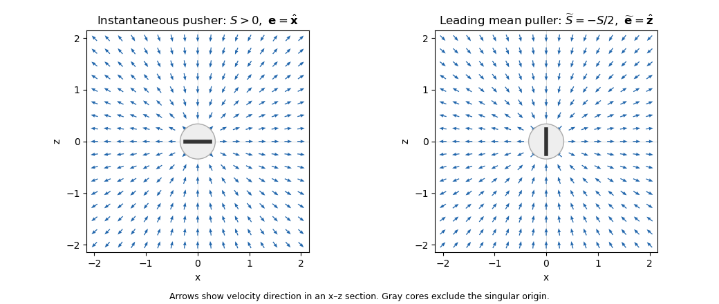
Writing $\cos \alpha =\mathbf{e}\cdot \hat{\mathbf{r}}$, its radial velocity isConsequentlyThis classifies pusher microswimmers and puller microswimmers in the force-on-fluid convention used by the given formula.

For the circular swimmer let $\phi =\omega t$, $\mathbf{p}=(\cos \phi ,\sin \phi ,0)$, ${\mathbf{x}}^{\prime }=R\mathbf{p}$, and choose the tangent director $\mathbf{e}=(-\sin \phi ,\cos \phi ,0)$. Its sign is immaterial to the stresslet. Write $\mathbf{r}=\mathbf{x}$ for the observation vector from the circle centre, and assume $r\gg R$. The leading far-field orbit average of a tangent stresslet is obtained by replacing $\mathbf{x}-{\mathbf{x}}^{\prime }$ by $\mathbf{r}$ while retaining the time-dependent director.

The orientation averaging of an axisymmetric stresslet over a full revolution givesSubstitution givesThuswith $\tilde{\mathbf{e}}$ equivalently $-\hat{\mathbf{z}}$. The effective axis is normal to the orbit plane. A positive original strength becomes negative, and a negative strength becomes positive: a pusher averages to a puller, and a puller averages to a pusher, at leading far-field order. The result is independent of $R$ and $\omega$ at this order.

The accuracy of the centre replacement can be made explicit. Half a revolution changes $\mathbf{p}$ and $\mathbf{e}$ to their negatives; the stresslet is even in $\mathbf{e}$. Pairing those times replaces the displaced field byHenceThe finite-radius average is not exactly a point stresslet at every location. For example, on the positive $z$ axis the exact average of the supplied model iswhich has the derived point-stresslet limit for $z\gg R$. This even displacement correction in an orbit-averaged stresslet is consistent with the far-field restriction.