The telescope forms the sky image at the entrance slit. A collimator makes the transmitted beam parallel, a reflection diffraction grating disperses it, and a camera’s optical lens focuses each wavelength to a different detector position.
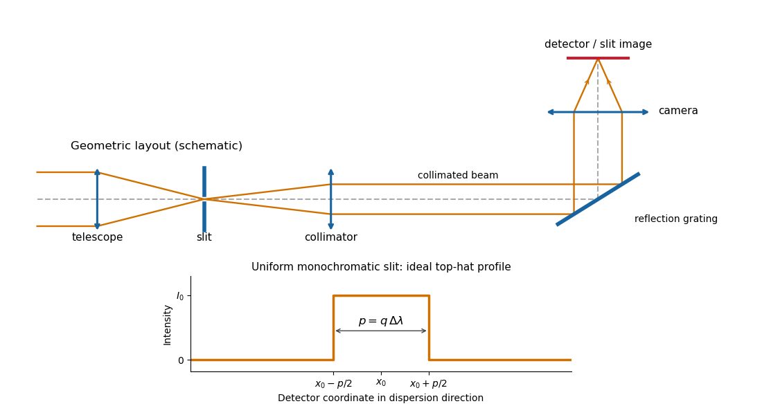
Reflection-grating spectrograph and slit-limited line profile
. Details. 
With a uniformly illuminated slit, ideal imaging and negligible slit diffraction, each monochromatic slit image has an approximately top-hat intensity profile of physical width . A small wavelength separation displaces two such images by , using the positive magnitude of grating dispersion. In the geometrical, slit-limited convention, resolution occurs when the displacement is of order the slit-image width. HenceHere is the slit’s apparent wavelength extent. A finite diffraction grating broadens the sharp edges; the top-hat sketch and the following identities presume slit-limited resolving power of a grating, rather than the regime where the grating’s own diffraction determines the line width. A precise resolution criterion for nonideal profiles can change order-unity factors.
Let the telescope and collimator have focal lengths , and let be the physical slit width. The collimated beam diameter in the dispersion direction is , so .
The diffraction grating changes both the angular width and the beam diameter. At fixed wavelength, differentiating the grating equation gives . Thus the anamorphic magnification of a grating givesIf is the illuminated surface length, its projected beam diameters are and . Multiplication cancels the anamorphic factors:ThereforeThis is a one-dimensional optical-invariant relation: a grating cannot independently magnify the slit and shrink the corresponding beam without compensating angular changes. The calculation uses local paraxial imaging about each instrument’s chief ray and an unclipped beam.
From the slit profile, the spectral resolving power obeys . Substitute into the preceding optical-invariant relation:The slit-image width cancels. Although is a detector length per unit wavelength, is a detector length, so this expression for has units of length, as does .
Use the signed-angle convention in which the reflection grating equation is , with positive diffraction order . For fixed incidence,The second identity is the local focal-plane scale, measured about the camera axis aligned with the central diffracted ray. Since , the projected beam size cancels the cosine in the grating dispersion:Writing for the number of illuminated grooves also gives . This connects the geometrical instrument invariant to the phase span of the illuminated diffraction grating.
Substitute the grating equation into the preceding result:Moving across the illuminated grating by one groove spacing changes the incident-plus-outgoing optical path length by . Across length , the total path difference is therefore . Thus is the optical path difference between contributions from the two ends of the illuminated grating.
The number of coherent phase cycles across it is , which is the intrinsic diffraction-limited spectral resolving power of the diffraction grating under the usual first-minimum criterion. In the slit-limited regime, also states how much sky angle can be accepted at a given resolution and aperture. Holding slit angle and resolution fixed while increasing telescope diameter requires a larger optical path span. The geometry gives ; large incidence and diffraction angles increase resolution per unit grating length, though grazing beams become impractical.
The slit equations do not imply unlimited resolution when tends to zero. Once is comparable to , finite-aperture diffraction matters and the actual resolving power is bounded by about .
An integral field spectrograph obtains spectra throughout a two-dimensional field instead of along one slit alone. Its reduced spectral data cube is : two coordinates locate a spatial sampling element and the third labels wavelength. One slice at fixed wavelength is an image; one column at fixed spatial position is an optical spectrum. The third axis is spectral, not a third spatial direction.
- A lenslet array divides the image into spatial elements. The spectrograph disperses each lenslet’s output into a microspectrum, with spacing and orientation chosen to avoid overlap.
- A lenslet array feeding optical fibers provides contiguous sampling; the fiber outputs are rearranged into a pseudo-slit for a conventional spectrograph.
- A bare optical fiber bundle samples the image and also reformats it into a pseudo-slit. Its packing fraction and coupling can leave spatial gaps or transmission losses.
- An image slicer divides the image into strips, then rearranges them end to end. Dispersion preserves position along each strip, and the reconstruction restores the second spatial coordinate.
- A scanning Fabry–Pérot interferometer or tunable narrow-band filter records a sequence of nearly monochromatic images, stepping the transmitted band to assemble the cube.
- Imaging Fourier transform spectroscopy records an interferogram at every spatial pixel while scanning optical path length difference. Transforming each interferogram supplies the spectral coordinate.
The first four are simultaneous spatially multiplexed grating arrangements. The last two deliver equivalent cube coordinates by scanning; they are imaging spectrometers rather than simultaneous grating integral-field units, and variability during the scan can corrupt the cube. Detector packing, sampling, calibration and throughput determine the practical tradeoffs.
In angular differential imaging, the instrument is operated in pupil tracking: its pupil and associated quasi-static speckle patterns remain nearly fixed on the detector, while the sky rotates with the parallactic angle. A reference stellar point spread function is formed from other exposures, preferably excluding frames where a companion remains at almost the same location. Subtract the reference from each exposure, then derotate the residuals into the sky frame and combine them. A companion adds coherently after derotation; the stellar residuals are reduced. This is the technique described in the original angular-differential-imaging analysis. At angular separation , the approximate displacement is , so useful diversity normally requires .
In simultaneous spectral differential imaging, acquire nearby spectral-band images simultaneously, for example with a beam splitter and filters or an integral field spectrograph. Stellar speckle patterns approximately move radially in proportion to wavelength. Rescale each image by and normalize the stellar flux before subtracting bands. The speckles then approximately align, while a companion at a fixed sky position moves in the rescaled coordinates. A companion absorption band can also distinguish its spectrum from the star: methane bands are useful for cool companions, as in the TRIDENT instrument description, but methane is not a universal companion property. Positional diversity scales as .
ADI uses sky rotation; SSDI uses simultaneous spectral diversity and wavelength scaling of stellar speckles.
Both methods reduce structured stellar residuals, rather than removing all noise. In angular differential imaging, changing atmospheric turbulence, imperfect adaptive optics, flexure and thermal drift change the point spread function between frames. The reference then fails to represent the instantaneous stellar field. Small sky rotation makes close companions contaminate their own reference, causing differential-imaging self-subtraction. Extended disks are especially susceptible; subtraction can alter shape as well as total flux. More images help independent photon shot noise, but do not necessarily average away correlated residuals.
Simultaneous spectral differential imaging avoids the time delay, but different channels have non-common-path wavefront errors. Chromatic optical aberrations, wavelength-dependent amplitude errors and out-of-pupil propagation prevent a perfect radial rescaling of speckle patterns. Filter throughput, detector calibration, image registration and atmospheric dispersion also leave subtraction residuals. Nearby bands align the stellar field better but give less positional diversity; wider separation gives more displacement but larger chromatic mismatch. A smooth-spectrum companion, or one too close for appreciable rescaled displacement, can undergo severe differential-imaging self-subtraction.
Artificial-companion injection through the complete processing pipeline and forward modelling can calibrate lost throughput and photometric or astrometric biases. They do not guarantee that every correlated residual is a real source. Independent epochs or spectral evidence remain valuable.
Reference mismatch produces residual speckles; source contamination produces self-subtraction and biased photometry.
Articles by others on the same topic
There are currently no matching articles.