Past exam of the mathematics course of the year 1 of the natural sciences course of the University of Cambridge / 2023 / Paper 1 / 20

For a differentiable objective $f$ and regular constraint $g=r$, a constrained stationary point satisfieswhere $\lambda$ is a Lagrange multiplier. Solve these equations for both the coordinates and $\lambda$.

Geometrically, the gradient $\nabla g$ is normal to the constraint level set when $\nabla g\ne 0$. Every feasible infinitesimal displacement $\mathbf{v}$ is tangent to that level set, so $\nabla g\cdot \mathbf{v}=0$. At a constrained stationary point, the directional change $\nabla f\cdot \mathbf{v}$ must also vanish for every such tangent displacement. Thus $\nabla f$ is normal to the same tangent plane and is a scalar multiple of $\nabla g$. This is the geometric basis of the Lagrange multiplier method.

For a second constraint $h=s$, with linearly independent vectors $\nabla g$ and $\nabla h$, the feasible tangent directions are perpendicular to both. Their normal space is the linear span of these two gradients, so introduce a second Lagrange multiplier:These equations find candidates; deciding whether they are maxima, minima or saddle points requires further analysis. Constraint points where the required gradient independence fails must be examined separately.

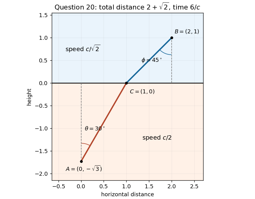
The angles in the PDF are measured from the vertical normal to the interface. The horizontal displacements of the two path segments are $d_1\tan \theta$ and $d_2\tan \varphi$, while their lengths are $d_1\sec \theta$ and $d_2\sec \varphi$. Thus the geometric constraint and travel time areThe Lagrange multiplier equations $\nabla T=\lambda \nabla g$ giveCancelling the positive geometric factors gives $\lambda =2\sin \theta /c=\sqrt{2}\sin \varphi /c$, henceThis is Snell's law, $\sin \theta /(c/2)=\sin \varphi /(c/\sqrt{2})$. The relation depends only on the ratio of the two speeds, so changing $D,d_1,d_2$ leaves the relation unchanged; it changes which angles satisfy it together with the geometric constraint.

For a minimum check, let $u$ be the horizontal distance to the crossing point. ThenandThus the travel time is a strictly convex function of $u$, and its stationary point is the unique global minimum. For positive $D,d_1,d_2$, $T^{\prime }(0)<0<T^{\prime }(D)$, placing the crossing between the two endpoint projections.

Put $s=\sin \theta$. By part (i), $\sin \varphi =\sqrt{2}s$. The acute-angle geometry requires $0<s<1/\sqrt{2}$. Expressing the tangents in terms of their sines in the geometric constraint gives the required implicit equationThe hint suggests $s=1/m$ for an integer $m\ge 2$. Testing $m=2$ givesThus $\boxed{\sin \theta =1/2}$. Each term on the left is strictly increasing in $s$ over the allowed interval, so this solution is unique.

The acute angles follow from part (ii) and the Snell's law relation:The path lengths below and above the interface are respectivelyHence the total distance and minimum travel time areFor a sketch to scale, choose the interface as $y=0$, with $A=(0,-\sqrt{3})$ and $B=(2,1)$. The crossing is $C=(1,0)$ because $d_1\tan \theta =d_2\tan \varphi =1$. The figure uses equal axis scales and shows the two normal-relative angles.