Put and , so the complementary probabilities are and . All four expressions are the row player's expected payoff, including those indexed by a column action. Direct expected value calculations giveThe column player's expected payoff is the negative of the row player's because this is a zero-sum game.
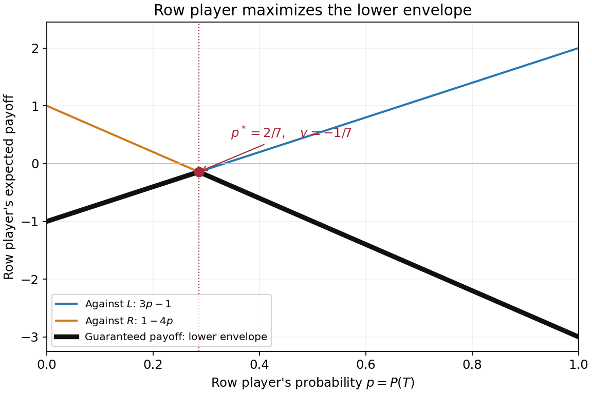
The bold black curve is the pointwise minimum of the two opposing-column expected payoff functions. It is the row player's security level payoff at the specified mixed strategy:The lines meet where , hence at . The first branch increases with slope and the second decreases with slope , so their intersection is the unique global maximum of the lower envelope:The endpoint values are and , both smaller. Since an opposing mixed strategy forms a convex combination of the two pure-column expected payoffs, it cannot make the row player's expected payoff lower than this envelope.
The bold black curve is now the pointwise maximum of the two pure-row expected payoff functions:It measures the largest expected payoff that the row player can achieve against column mixed strategy . The column player minimizes this quantity because its own payoff has the opposite sign. Equality of the two lines gives , or . The envelope decreases before that point and increases afterwards, givingThe endpoint values and are both larger. A row mixed strategy cannot exceed the greatest pure-row expected payoff, because its expected payoff is a convex combination of those two values.
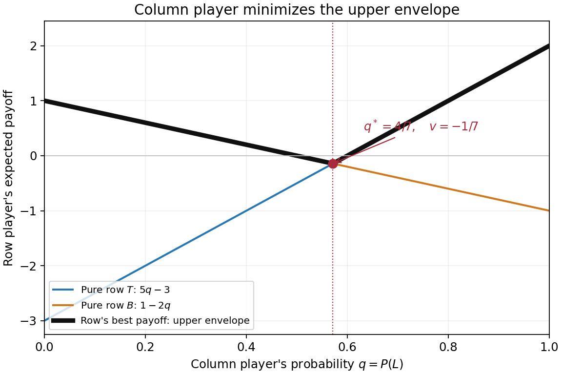


The unique Nash equilibrium uses row probabilities on and column probabilities on . The value of a zero-sum game to the row player is ; the column player receives .
The first graph solves the row player's max–min optimization: choose a mixed strategy guaranteeing the greatest possible worst-case expected payoff. The second solves the column player's min–max optimization: choose a mixed strategy placing the smallest upper bound on the row player's expected payoff. Their optimal heights agree, illustrating the minimax theorem.
There is also a direct Nash equilibrium certificate, so the conclusion does not depend on reading coordinates from a plot. At , both opposing pure columns give row expected payoff ; at , both pure rows give row expected payoff . By linearity, every unilateral deviation, including an arbitrary mixed strategy, leaves the deviator's expected payoff unchanged against the fixed opposing equilibrium mixture. Neither player can improve it. This is a mixed-strategy optimality certificate for a matrix game.
The equilibrium outcome is a probability distribution over cells, rather than one deterministic cell. Independent randomization givesThe resulting row expected payoff is . Finally, each envelope has a unique optimum, so any Nash equilibrium must use the displayed optimal mixed strategies. In particular there is no pure strategy Nash equilibrium.
Articles by others on the same topic
There are currently no matching articles.