Source paper: released examination archive.
By the Von Neumann-Morgenstern utility theorem, use a representing utility function and apply a positive affine function to set and . This is possible because the given strict preference implies . The two specified indifference relations then giveTaking the expected utility of each lottery yieldsTheir difference is , establishing the stated strict preference. These numbers measure utility, not monetary reward or an assumed ordering of the subscripts.
Here is the underlying argument directly in terms of the axioms. The independence axiom for lottery preferences permits substitution of indifferent lotteries inside a common mixture. Replacing by its given mixture of , and then replacing , followed by reduction of compound lotteries, givesand consequentlyThe transitive relation axiom combines the successive substitutions. Finally, mixture monotonicity says that among mixtures of a strictly better and a strictly worse outcome, the greater probability of the better outcome is strictly preferred; this follows from the independence axiom for lottery preferences and transitivity. Since and , the comparison follows. Complete lottery preferences and continuity of lottery preferences are part of the representation theorem's hypotheses; the direct substitution calculation uses the already supplied indifferences and does not need to invoke continuity of lottery preferences again.[ref]
Expected utility theory by EconPort. “The Expected Utility Property” and the preceding preference axioms
No: these two strict comparisons violate the independence axiom for lottery preferences. Let denote the certain zero-money lottery. Reduction of compound lotteries givesFor example, the second expression assigns probability to the nonzero reward and to zero. The claimed must therefore implywhich is , contradicting the other claimed strict preference.
The same obstruction is visible in any proposed expected utility representation. Subtract from the utility function, and write and . The first comparison requires , hence , whereas the second requires . No real satisfy both. This argument requires neither risk neutrality nor an assumption that the utility function is increasing in money.
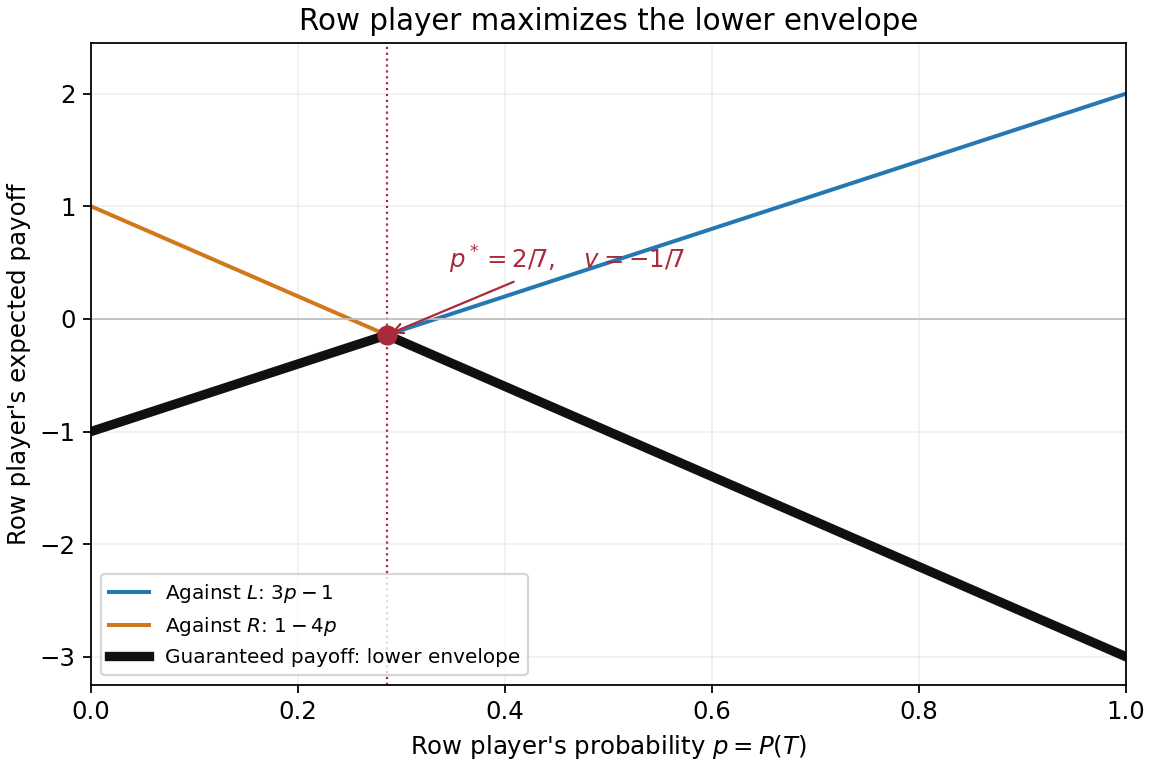
Put and , so the complementary probabilities are and . All four expressions are the row player's expected payoff, including those indexed by a column action. Direct expected value calculations giveThe column player's expected payoff is the negative of the row player's because this is a zero-sum game.
The bold black curve is the pointwise minimum of the two opposing-column expected payoff functions. It is the row player's security level payoff at the specified mixed strategy:The lines meet where , hence at . The first branch increases with slope and the second decreases with slope , so their intersection is the unique global maximum of the lower envelope:The endpoint values are and , both smaller. Since an opposing mixed strategy forms a convex combination of the two pure-column expected payoffs, it cannot make the row player's expected payoff lower than this envelope.
The bold black curve is now the pointwise maximum of the two pure-row expected payoff functions:It measures the largest expected payoff that the row player can achieve against column mixed strategy . The column player minimizes this quantity because its own payoff has the opposite sign. Equality of the two lines gives , or . The envelope decreases before that point and increases afterwards, givingThe endpoint values and are both larger. A row mixed strategy cannot exceed the greatest pure-row expected payoff, because its expected payoff is a convex combination of those two values.
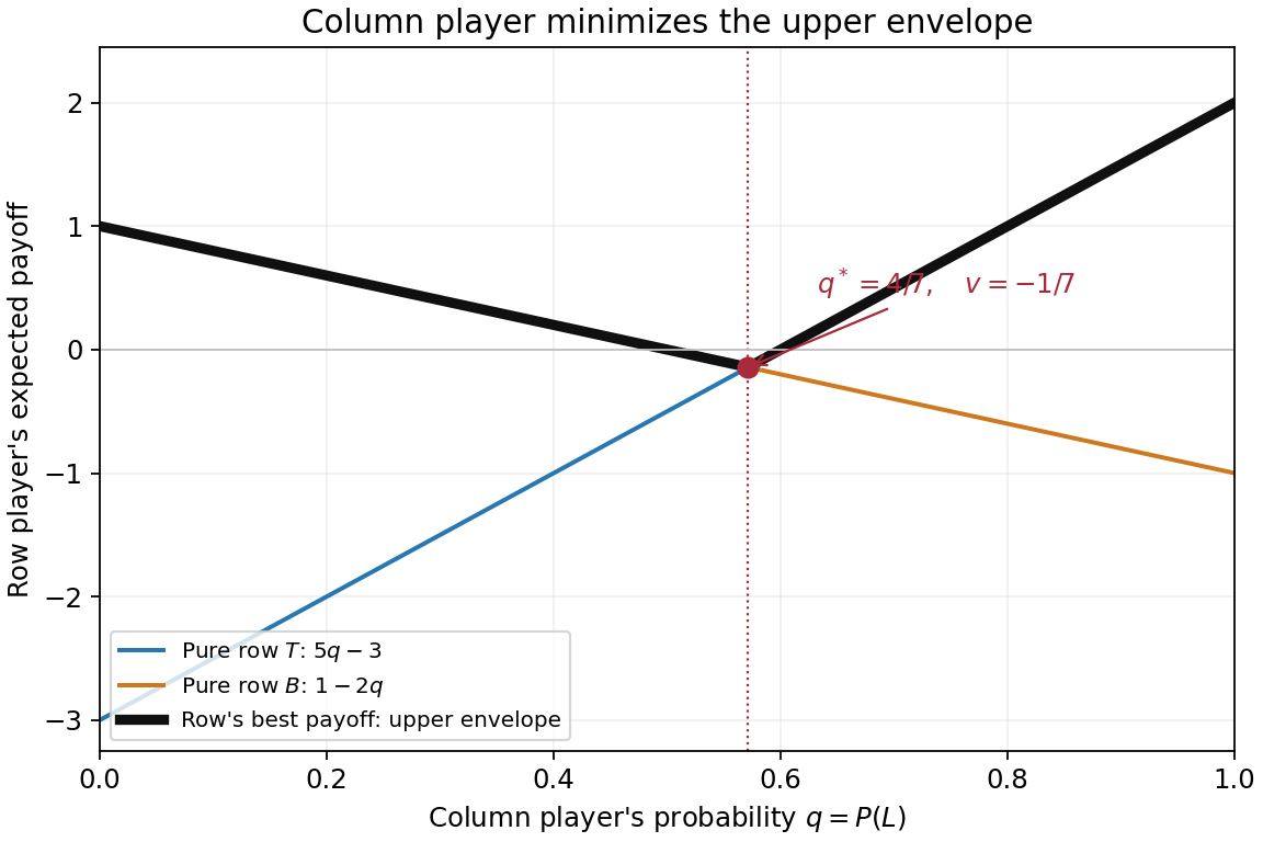
The unique Nash equilibrium uses row probabilities on and column probabilities on . The value of a zero-sum game to the row player is ; the column player receives .
The first graph solves the row player's max–min optimization: choose a mixed strategy guaranteeing the greatest possible worst-case expected payoff. The second solves the column player's min–max optimization: choose a mixed strategy placing the smallest upper bound on the row player's expected payoff. Their optimal heights agree, illustrating the minimax theorem.
There is also a direct Nash equilibrium certificate, so the conclusion does not depend on reading coordinates from a plot. At , both opposing pure columns give row expected payoff ; at , both pure rows give row expected payoff . By linearity, every unilateral deviation, including an arbitrary mixed strategy, leaves the deviator's expected payoff unchanged against the fixed opposing equilibrium mixture. Neither player can improve it. This is a mixed-strategy optimality certificate for a matrix game.
The equilibrium outcome is a probability distribution over cells, rather than one deterministic cell. Independent randomization givesThe resulting row expected payoff is . Finally, each envelope has a unique optimum, so any Nash equilibrium must use the displayed optimal mixed strategies. In particular there is no pure strategy Nash equilibrium.
Exactly , and can be sustained as constant stage game outcomes. Their long-run average payoffs are , and , respectively. We assume the usual repeated game monitoring convention: both players observe each completed joint action before the next round. The source's colour convention puts the blue lower-left row payoff first and the red upper-right column payoff second.
For necessity, row action earns against , so playing it forever guarantees a nonnegative long-run average payoff against every opposing pure strategy. Similarly, column action earns against and guarantees zero or more. Conversely, column action holds the row player's best possible stage payoff to , and row action holds the column player's to . Thus each player's minmax payoff is exactly .
Any Nash equilibrium must give both players at least zero, an individually rational payoff in a repeated game. Every off-diagonal cell has a negative payoff for one player: and hurt row, and hurt column, hurts row and hurts column. Repeating any such cell forever therefore permits a profitable unilateral deviation to the zero-guaranteeing action. The three diagonal cells pass this necessary test.
For sufficiency, fix target or . Each player's finite-state strategy has initial state and an absorbing state . In , output the player's component of ; remain in if the completed joint action equals , and otherwise move to . In , row always outputs and column always outputs , regardless of further observations. These are two-state grim trigger strategies; the separate machines are drawn below. The input is the observed joint action, so after any off-path history the prescribed continuation states agree.
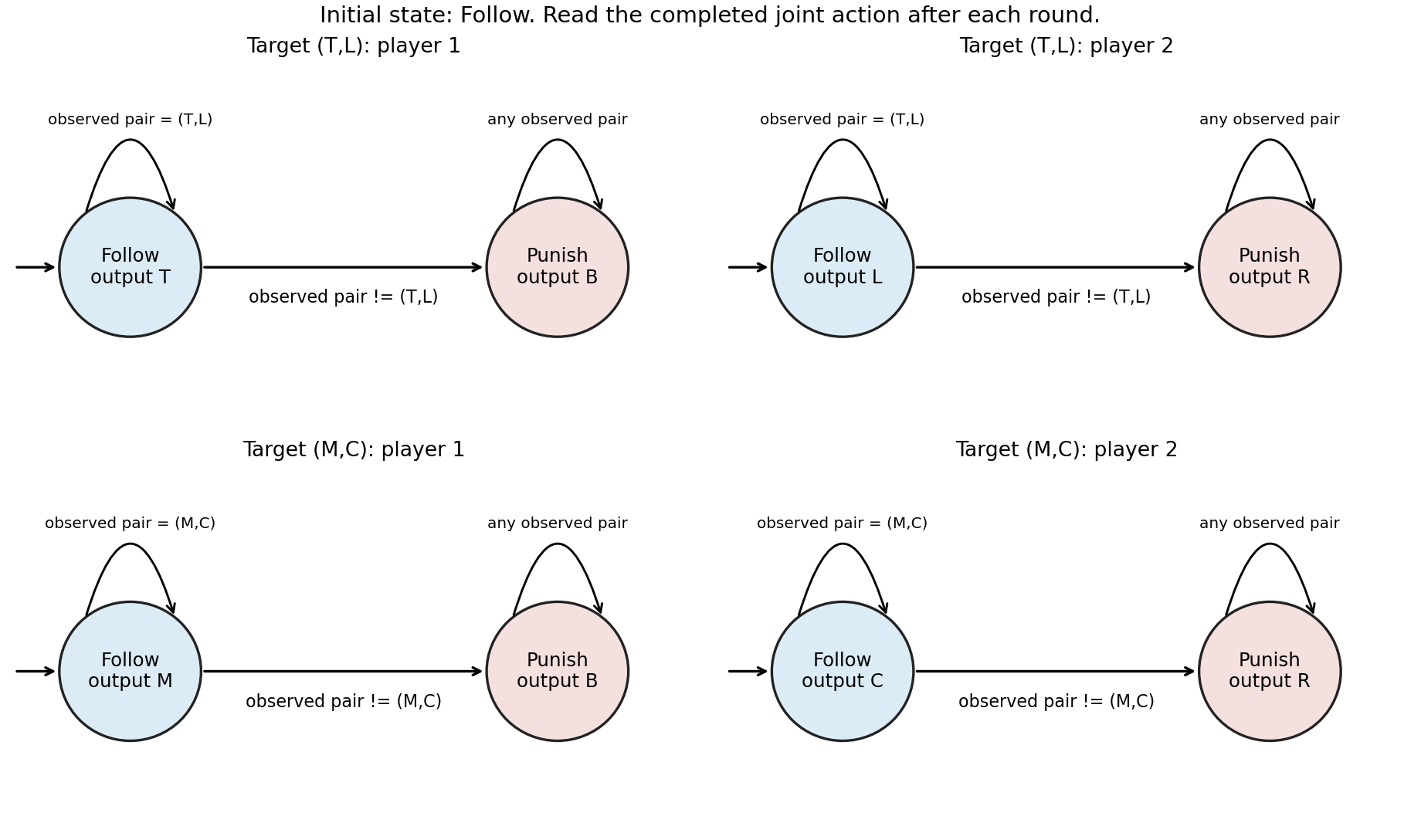


If neither player deviates, the target is repeated forever. If a player first deviates at a finite round , the opponent enters for all later rounds. Against column action , every row action earns at most zero; against row action , every column action earns at most zero. All payoffs are bounded, so the total reward before and at , divided by the horizon, tends to zero. The deviator's upper limiting average is therefore at most , below either target payoff or . This proof tests arbitrary future deviations, not merely a single changed action. It also rules out improvement by deviations whose averages fail to converge, if the criterion is extended by an upper or lower limit.
For target , one-state machines outputting and forever suffice: each is a best response to the other in every round. Their long-run average payoffs are zero and no unilateral deviation can improve them. In fact, the punishment is credible because is a stage Nash equilibrium, so the two positive-target constructions are also subgame perfect equilibria under the stated monitoring assumption. The general punishment mechanism is described in [ref]
Lecture 15: Repeated Games by Asu Ozdaglar. slides 12–15; those slides use discounting, while the finite-prefix argument here uses long-run averages
.“Outcomes of the stage game” here means a fixed action pair repeated forever. Allowing time sharing also sustains some average payoff vectors that are not stage cells: for example, a deterministic alternating cycle gives , with a two-phase finite-state strategy and the same permanent punishment. An off-diagonal cell may occur in a sustainable cycle; the impossibility above concerns its constant repetition, not every appearance on an equilibrium path. With finite-state pure strategies, an undisturbed path is eventually periodic, so its limiting cell frequencies are rational numbers.
Use the standard repeated game convention that the first round's joint action is observed before round two. The following original game tree represents simultaneous moves by making row move first in each round while hiding that current move from column. Terminal labels are total payoffs over both rounds, ordered row then column.
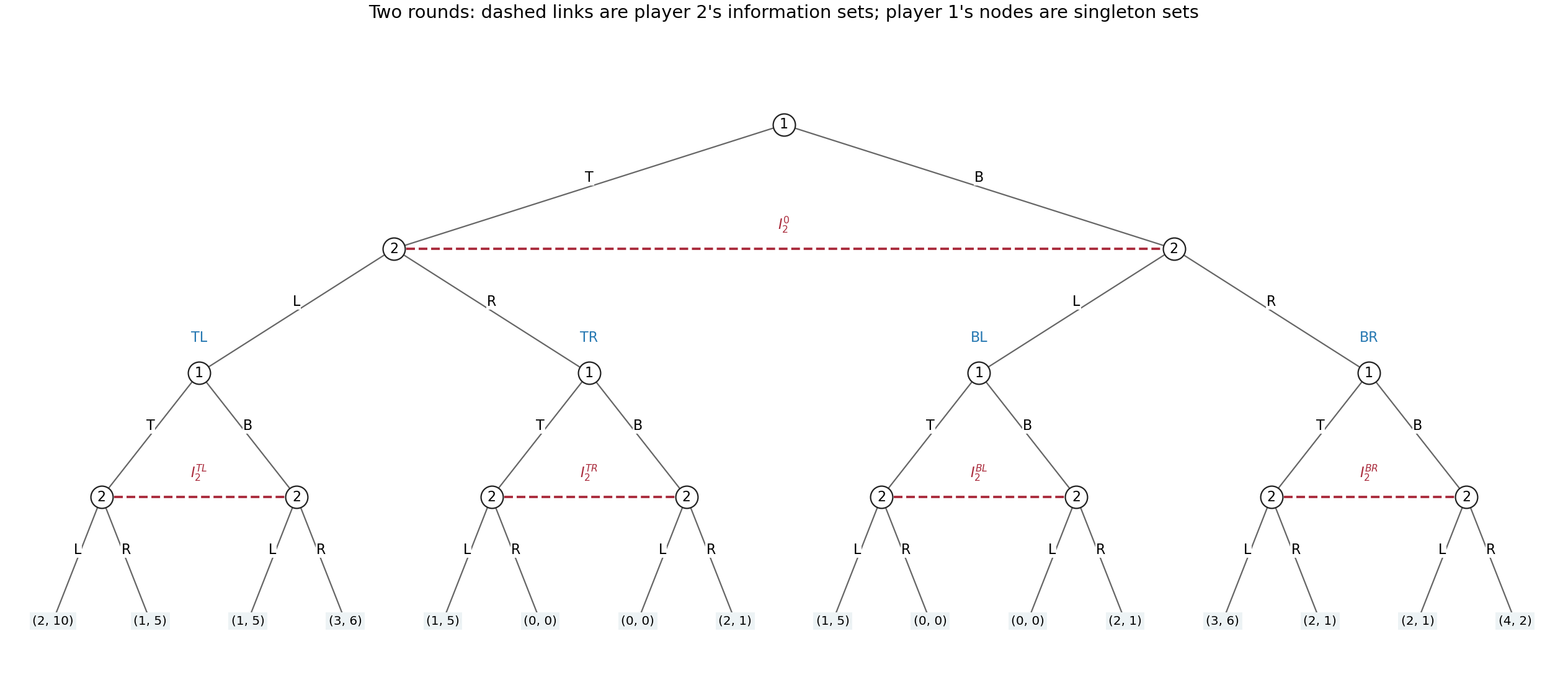
The full two-round extensive-form game, with all sixteen terminal payoff pairs and five column information sets
. Details. 
Formally, round one starts at a row decision with actions . The two ensuing column nodes form one information set , with available actions ; column cannot tell which current row action occurred. The four completed first-round histories are . At each , round two begins at a separate row node. Its two successors, after row's current or , form a column information set . Distinct have distinct information sets: both players know the whole first-round outcome. There are sixteen terminal histories , whose total payoff is , as displayed in the tree.
The row player's five information sets are the initial singleton and the four singleton round-two nodes, one per . The column player's five information sets are and the four two-node sets . Thus each player must specify one binary choice at each of five information sets, including histories that its own first choice might prevent:Counting only the four possible two-round action sequences would miss the distinct contingent responses to the opponent's first action.
For a concrete pair of complete pure strategies, order the second-round histories as and useThe first entry is the initial action, and the four remaining entries prescribe the action after each first-round history. This induces the unique path in round one followed by in round two. Hence the total payoff isThe off-path entries are part of each pure strategy, even though this pair does not reach them.
For randomization, a mixed strategy is a probability distribution over the complete plans, with free probabilities in a general distribution. A behavioural strategy instead gives one binary-action probability at each of five information sets, requiring five parameters. This game has perfect recall: a player never forgets a previous own action or a first-round observation, and the only concealed action is the opponent's current simultaneous choice. Consequently neither kind of randomization has a greater attainable-payoff advantage: Kuhn's theorem gives realization-equivalent strategies against every fixed opposing strategy.[ref]
Extensive games and the problem of information by Harold W. Kuhn. original article, pp. 193–216, equivalence under perfect recall
The equivalence can be verified directly here. Given a behavioural strategy, sample all five contingent actions independently before play; the resulting product probability distribution over complete plans is an equivalent mixed strategy. Conversely, let be a mixed strategy for player . Use its marginal probability for the initial action. At history containing own first action , choose second action with conditional probabilitywhenever the denominator is positive; if it is zero, choose arbitrarily at that unreachable history. The opponent's first-round action is simultaneous and cannot depend on the sampled hidden plan beyond the chosen first action. Thus conditioning on preserves exactly these conditional probabilities of actions, and multiplying the first- and second-round factors reproduces each terminal probability. Correlations between prescriptions at mutually exclusive second-round histories have no further observable effect. Behavioural strategies offer the more compact representation, while mixed strategies describe a single random choice of a full plan. Imperfect information here does not mean imperfect recall.
If the core is nonempty, it is exactly the singleton allocation for every . Take any in the core of a cooperative game and write . Core membership gives efficiency of the imputation, , and the coalition inequalitiesUsing the given complementary-coalition equality in this constant-sum cooperative game, the second inequality yieldsCombining upper and lower bounds gives for every coalition . In particular,Since this holds for any core member and at least one exists by hypothesis, the displayed allocation is in the core and is its only member. The argument also shows why nonemptiness is restrictive: it forces for every coalition, so the characteristic function of a coalitional game must be additive. No superadditive coalitional game or monotonicity assumption is needed.
cannot have an induced subgraph game representation. is represented by a weighted triangle with edge weights , , , and has Shapley value vector .
In an induced subgraph game, players are graph vertices and a coalition receives the sum of the weights of graph edges whose two endpoints lie in it. Therefore each two-player coalition determines the corresponding edge weight. For these weights would have to be , making the grand coalition worth , whereas its actual value is . No other edge weights can repair that discrepancy without changing a two-player coalition's value. Even a convention allowing vertex weights would not help: its singleton values force all such weights to zero.
For , the stated weighted graph triangle has grand coalition value and reproduces all three pair values. Empty and singleton coalitions contain no graph edges, so their values are zero. This verifies all eight coalitions and supplies the complete representation.
To compute the Shapley value, reveal players in a uniformly random permutation. An edge's weight contributes to an endpoint's marginal contribution precisely when the other endpoint appeared earlier. Each endpoint is later with probability , independently of where the third player appears. Linearity of the expected value therefore splits each edge weight equally between its two endpoints:The values sum to , as required by the Shapley value's efficiency property. This is the general Shapley value of an induced subgraph game formula, not an assumption that all three players are symmetric: player has a different incident-weight total.
The core is the singleton . Here the characteristic function of a coalitional game is , the two-person instance of the core of the miners game calculation.
Let be in the core. Efficiency requires , and every pair coalition requires . Summing the six pair inequalities counts each coordinate three times, giving . Efficiency makes this an equality; since every individual slack is nonnegative, all six pair inequalities must be equalities. In particular forces , and comparison with gives every .
Conversely, for the uniform allocation every coalition satisfiesand its total is . It is therefore a core member, completing both existence and uniqueness. In particular, a three-player coalition receives ; the pair constraints are the tight ones.
The core is empty. Efficiency would require . Each two-player coalition has value , so core membership would also requireAdding gives , contradicting efficiency, which makes the left side . Thus no allocation can meet all coalition demands. The obstruction uses only pair coalitions and the grand coalition; imposing individual rationality cannot remove it. The equal allocation is efficient but gives each pair only , so symmetry does not supply a core allocation.
Articles by others on the same topic
There are currently no matching articles.