Use the normalized local truncation errorThe Taylor theorem expansions about areSubstitution gives exactlyThus the theta method has order two exactly for , and otherwise order one, as a statement about the method on a sufficiently smooth class of problems. The leading term vanishes at one half, and a function with nonzero third derivative shows that the next term does not vanish universally. As usual, a uniform order estimate assumes bounded relevant derivatives; mere existence of on the open interval gives the stated pointwise remainders but not, by itself, a uniform bound. Special exact solutions can of course have zero truncation error even for a first-order method.
Put . Subtracting the numerical update from the exact update with its local truncation error givesThe Lipschitz condition in the solution variable and the triangle inequality implyThe assumed positive denominator permits division. With and , repeated substitution of this Lipschitz one-step error bound yieldsHere because , so the displayed geometric series quotient is well defined. For implicit steps, the same condition makes the scalar update map a contraction mapping, ensuring a unique numerical next value.
On the Dahlquist test equation, set . The theta method has stability functionWith the decaying-solution convention, its region of absolute stability is . Writing , squaring numerator and denominator givesFor this is the open disk with centre and radius . At it is the open left half-plane. For it is the exterior of the closed disk with centre and radius . The pole , when present, lies outside the stability region.
Every with satisfies the inequality exactly for . If , sufficiently large negative real fails it. ThereforeIf absolute stability is instead defined by bounded amplification, the boundary is included; this convention does not change the A-stability conclusion for the open left half-plane.
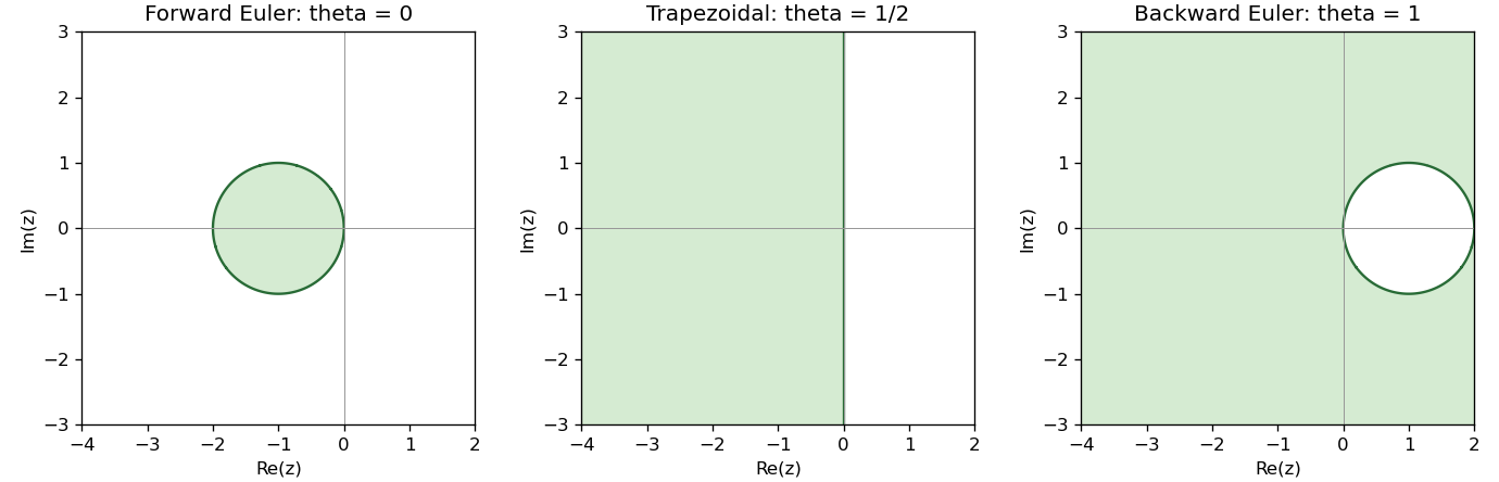
Absolute stability regions of the theta method at zero, one half and one; green regions damp the scalar test solution
. Details. 
In the normalization used by the supplied coefficient expansion, the local truncation error of the linear multistep method isThe nonzero sum in the denominator is an explicit hypothesis. Consistency of a numerical method requires uniformly on a fixed finite time interval for every sufficiently smooth exact solution as . Equivalently, the two polynomial identities areThese follow by inserting constant and affine functions, or by setting the first two Taylor coefficients to zero.
Zero-stability means that perturbations of the starting values of the zero-step recurrence remain bounded by a fixed multiple of their initial size, uniformly as the number of steps tends to infinity on a fixed time interval. In particular solutions of obey with independent of .
The equivalent root condition for a multistep method isA root outside the unit circle gives exponential growth of a recurrence relation mode; a repeated root on it gives polynomial growth. Repeated roots strictly inside it are harmless because their polynomial factor is dominated by decay.
The first characteristic polynomial factors asThe two quadratic roots have product one. Both can lie in the closed unit disk only if both have modulus one, requiring . At the root one is triple and ; at the root minus one is double. Both fail the root condition for a multistep method. In the intervening open interval the two quadratic roots are distinct conjugate unit-modulus roots, different from one. ThusUsing , the supplied expansion givesThroughout the zero-stable range, , so every such method has order two. There is a unique higher-order choice:Here and , giving exactly order four, with normalized leading truncation error . But the extra roots are , one of modulus greater than one. By the Dahlquist equivalence theorem this consistent but non-zero-stable method is not convergent for arbitrary consistent starting values.
Let , and define analogously. The Crank-Nicolson diffusion scheme isUse and zero values on every boundary node for every time level. This is the theta method with applied to the spatial finite difference method for the heat equation.
Write . The update can be rearranged asWhen , the right side is a convex combination of old values: its coefficients are nonnegative and sum to one. Assume all old values lie in . A new maximum is interior because boundary values are zero and . At its node the left side is at least , while the right side is at most , a contradiction. A new minimum similarly makes the left side at most and the right side at least , again a contradiction.
The initial values satisfy the bounds by construction; mathematical induction provesThe new-time matrix is a strictly diagonally dominant matrix with positive diagonal and nonpositive off-diagonal entries, so the linear update is uniquely solvable. This Crank-Nicolson maximum principle under a step restriction concerns preservation of value bounds, which is a stronger requirement than scalar A-stability.
For nonnegative initial data, . The proved Crank-Nicolson maximum principle under a step restriction immediately gives for all indices. For nonpositive initial data, and the same bound gives . Equivalently, apply positivity to , since the finite difference method is linear and has homogeneous Dirichlet boundary conditions. Both conclusions use .
Articles by others on the same topic
There are currently no matching articles.