Eight units; extended essays or structured projects may replace some written units. Optional branches are a verified selection.
The initial table of content was limited to the first level because it is larger than 1000 articles. There are 1377 articles in total. Expand a branch to load its children.
Original solutions to past examinations of the graph theory course of the University of Oxford.
Solutions to all three questions of the graph theory course of the University of Oxford Part B examination, sat on 15 June 2023. Source: original released PDF, bundle pages 243–244; paper pages 1–2. Throughout, graphs are finite simple graphs unless a construction explicitly permits parallel edges.
A proper edge colouring assigns colours to the edges of a graph so that distinct edges sharing a vertex have different colours. The edge chromatic number is the least number of colours in such an assignment. Equivalently, it is the least number of matchings in a graph whose disjoint union is the entire collection of edges.
Vizing's theorem states that a finite simple graph of maximum degree satisfiesThe lower bound holds because all edges incident with a vertex of vertex degree require different colours.
Hall's marriage theorem states that a finite bipartite graph with vertex sets has a matching in a graph saturating if and only ifwhere is the graph neighbourhood of . Here matching saturation means that each vertex of is incident with an edge of the matching in a graph; it does not require every vertex of to be met.
Let . Apply Hall's marriage theorem to the induced subgraph on , which is a bipartite graph. For any subset , double counting the edges from to its graph neighbourhood givesThe equality uses the fact that every neighbour of lies in , so all edges incident with have been counted. The final inequality uses the maximum degree bound on . Since , division gives the Hall condition .
Consequently there is a matching in a graph saturating . If is empty, use the empty matching in a graph. This proves the required matching covering maximum-degree vertices in a bipartite graph on the specified side; other vertices need not be met.
By part (i), choose a matching in a graph meeting all vertices of vertex degree in . Interchanging the two vertex sets gives a matching in a graph meeting all such vertices in . Consider the spanning subgraph with edges .
Every vertex has vertex degree at most two in . An edge belonging to both matchings in a graph forms a whole two-vertex connected component of a graph, since neither endpoint can meet another edge of either matching in a graph. On every other nontrivial connected component of a graph, the edges alternate between and , so the connected component of a graph is a graph path or an even graph cycle. We select one of the two matchings in a graph separately on each connected component of a graph.
On a graph cycle, either choice covers every vertex. On a graph path with an odd number of edges, the first and last edges belong to the same matching in a graph; choose it, and it covers every vertex of the graph path. For a common edge, choose that edge.
It remains to treat a graph path with a positive even number of edges. Its endpoints lie in the same side of the bipartite graph. Every internal vertex meets both matchings in a graph. If both endpoints lie in , choose : every endpoint of vertex degree must already be met by , by its defining property. If both endpoints lie in , choose for the same reason. Thus the choice meets all vertices of vertex degree in that connected component of a graph.
Finally, an isolated vertex of cannot have vertex degree in , since it would have been met by or . The union of the selected edges over the connected components of a graph is a matching in a graph, because different connected components of a graph have disjoint vertex sets. It meets every vertex of vertex degree in . The useful mechanism is the union of two matchings and its alternating connected components of a graph.
Use mathematical induction on the maximum degree , including as the base case. A graph of maximum degree zero has no edges, so zero colours suffice.
For , part (ii) supplies a matching in a graph meeting every vertex of vertex degree . Delete its edges, retaining all vertices. Each vertex formerly of maximum degree loses one incident edge; every other vertex already had vertex degree at most . HenceThe resulting graph is still a bipartite graph. By mathematical induction, it has a proper edge colouring using at most colours. Give every edge of one new colour. Since is a matching in a graph, this produces a proper edge colouring of with at most colours. The edges at a vertex of maximum degree require at least colours, soThis is Kőnig's line colouring theorem.
For even , take the complete graph . It is an -regular graph on an odd number of vertices. Every matching in a graph has at most edges, so colours in a proper edge colouring could cover at most edges. ButTherefore ; Vizing's theorem gives . This includes the graph triangle when .
For odd , first construct a graph on vertices. Start with the complete graph onand delete the edges , , and . The pairing is possible because is even. In the initial complete graph, every vertex has vertex degree . The distinguished vertex loses two edges and every other vertex loses exactly one, givingTake two disjoint copies of , with distinguished vertices , and add the edge . The resulting simple graph is an -regular graph. The added edge is the only edge between the two copies; each copy has the odd number of vertices.
Suppose an -colour proper edge colouring existed. At each vertex, the incident edges would use all colours. Thus each colour would form a perfect matching. Any perfect matching must use : without it, each odd-sized copy would have to be covered by internal pairs, which is impossible by parity. Therefore all colour classes would have to contain the same edge , a contradiction. Hence Vizing's theorem again givesThese constructions give class two regular graphs for every . The odd- construction exhibits the bridge obstruction to regular edge colouring; is a connected graph because every vertex other than is adjacent to , while are adjacent to those vertices.
For a finite graph , its chromatic polynomial is the polynomial whose value at each positive integer counts proper vertex colourings of from a fixed palette of labelled colours. Adjacent vertices must receive different colours, and unused colours are allowed.
For an edge , the deletion-contraction recurrence for the chromatic polynomial isHere deletes only the edge , while performs edge contraction, identifying and removing . Any parallel edges produced by edge contraction can be replaced by a single edge, since their constraints on proper vertex colourings are identical.
Indeed, the proper vertex colourings of in which differ are precisely those of , while those in which agree correspond bijectively to proper vertex colourings of . This proves the equality for every positive integer , hence as a polynomial identity. Together with for a graph without edges, the recurrence also proves by mathematical induction that the counting function is a polynomial.
Let the nonempty connected components of a graph of be . A proper vertex colouring can be chosen separately on each connected component of a graph, since no edge joins different connected components of a graph. The multiplication principle gives, first at positive integers and then as a polynomial identity,It remains to justify that every factor has zero constant term. More generally, for every nonempty simple graph , prove by mathematical induction on the number of edges. If there are no edges, then with . Otherwise choose an edge . Both and the simplified edge contraction are nonempty graphs with fewer edges. The deletion-contraction recurrence for the chromatic polynomial and mathematical induction giveThus for a polynomial , andFor the empty graph, and , so the conclusion also holds. This is the chromatic polynomial product over components.
Write and . For , let denote the number of connected components of a graph of the spanning subgraph , including isolated vertices. The inclusion-exclusion principle, applied to the unwanted events that the two endpoints of an edge receive the same colour, gives the chromatic polynomial inclusion-exclusion formulaTo justify the exponent, imposing equal colours across all edges in forces a single colour on each connected component of a graph of , with independent choices between its connected components of a graph. Thus the corresponding count at colours is . Equality for all positive integers proves the polynomial identity.
Fix an index in the stated range. A subset contributes to the coefficient of exactly when . If contains a graph cycle of length , the hypothesis gives . All its vertices lie in one connected component of a graph. For any connected component of a graph , its contribution to is , soThis contradicts . Therefore every contributing is a forest. The forest identity then gives .
Conversely, every -edge subset is a forest, since a graph cycle in it would have at most edges. It therefore has and contributes exactly . There are such subsets, by the definition of a binomial coefficient. ConsequentlyHere the coefficient notation is understood within the defined indices ; if the displayed range is extended past , the coefficients beyond the constant term can be set to zero. For a forest, , so the binomial coefficients there are also zero. The key reason girth determines initial chromatic coefficients is that a graph cycle can affect only exponents whose loss of connected components of a graph is at least .
First reduce the unicyclic graph to its unique graph cycle . Delete the edges of but retain every vertex. The remaining graph is a forest, since any surviving graph cycle would be a second one in . Each of its connected components of a graph contains a vertex of : follow a graph path to in the original connected graph, stopping at the first vertex of ; this initial segment uses no edge of .
No such connected component of a graph contains two vertices of . Otherwise, on the tree graph path between them, choose two successive visits to . The segment between these visits has no internal vertex on and uses no edge of . Combining it with either connecting arc of gives a second graph cycle, a contradiction. Thus the remaining graph consists of trees, each rooted at exactly one vertex of .
After choosing a proper vertex colouring of from colours, colour these rooted trees away from their roots. Each of the off-graph cycle vertices has one already coloured parent in a rooted tree, leaving exactly choices. The multiplication principle therefore givesEquivalently, this repeatedly applies the chromatic polynomial after attaching a leaf formula.
To compute the chromatic polynomial of a cycle, the base case is the graph triangle:For , deleting a cycle graph edge gives a path graph on vertices, while edge contraction gives . The chromatic polynomial of that path graph is , by choosing the colour of its first vertex and then each successive vertex. Hence the deletion-contraction recurrence for the chromatic polynomial givesUsing mathematical induction, substitute to obtainMultiplying by the factor for the attached trees proves the chromatic polynomial of a unicyclic graph formula
A graph is a k-connected graph if it has at least vertices and deleting any set of fewer than vertices, together with their incident edges, leaves a connected graph.
The vertex connectivity is the largest such . Equivalently, for a graph with at least two vertices, it is the smallest number of vertices whose deletion either disconnects the graph or leaves a single vertex. The latter convention gives for a complete graph. A disconnected graph has vertex connectivity zero; one usually also sets .
For distinct nonadjacent vertices , the local connectivity isSuch a set is an – vertex separator. By Menger's theorem, local connectivity also equals the maximum number of internally vertex-disjoint paths from to . If no graph path exists already, the empty vertex separator gives zero.
The vertex separator version of Menger's theorem says that, for distinct nonadjacent vertices of a finite graph, the maximum number of internally vertex-disjoint paths from to equals the minimum size of an – vertex separator.
Use the following version of the max-flow min-cut theorem: in a finite directed flow network with nonnegative integer flow network edge capacities, the maximum flow value equals the minimum cut capacity, and a maximum flow can be chosen to have integer values on every directed edge. The last clause is the integral max-flow theorem.
Here is the reduction, including the correspondence with vertex separators. Put . Perform vertex splitting on each vertex , replacing it by with a directed edge of flow network edge capacity one. Keep as the source and as the sink. For each original undirected edge , put directed edges from the output of to the input of and from the output of to the input of , each of flow network edge capacity ; an unsplit endpoint uses or itself.
A family of internally vertex-disjoint paths gives a feasible integral flow of value , by sending one unit down each graph path. Conversely, decompose an integral flow into unit source-to-sink graph paths and directed cycles, discarding the directed cycles. This decomposition can be obtained by following positive-flow directed edges and subtracting one unit along a source-to-sink graph path or a directed cycle, repeating until the flow value is exhausted. A capacity-one split edge can belong to at most one unit graph path. The projected graph paths in are therefore internally vertex-disjoint paths. Thus the largest number of such graph paths equals the maximum flow value.
Deleting a vertex separator corresponds to removing its split edges, of total flow network edge capacity . This destroys every source-to-sink graph path; taking the source-reachable vertices after removal gives a cut of a flow network of cut capacity at most . Thus the minimum cut capacity is no greater than the minimum vertex separator size.
For the reverse inequality, deleting all internal vertices separates , because they are nonadjacent. Hence a minimum cut has cut capacity at most and cannot contain a directed edge of flow network edge capacity . Its outgoing edges are therefore split edges. Let be the original vertices associated with them. Any – graph path avoiding would lift to a source-to-sink graph path crossing this cut of a flow network without using an outgoing edge, an impossibility. Hence is a vertex separator, with size exactly the cut capacity. The two minima agree, and the max-flow min-cut theorem proves Menger's theorem.
Add two new vertices to , joining to every vertex of and to every vertex of , with no other new edges. The vertices are nonadjacent. Suppose has . Since is a k-connected graph, is a connected graph. Both and are nonempty because each original set has cardinality . Choose and ; a graph path between them in extends to an – graph path avoiding .
Consequently no fewer than vertices can form an – vertex separator. By Menger's theorem, there are at least internally vertex-disjoint paths from to . There cannot be more than , since has only neighbours.
Remove from these graph paths. The resulting graph paths in start at distinct vertices of , end at distinct vertices of , and are pairwise vertex-disjoint paths: any shared vertex would have been an internal vertex common to two of the original graph paths. Because there are exactly graph paths, they use every vertex of and as an endpoint. None can pass through another terminal internally, since that terminal already occurs as an endpoint of one of the vertex-disjoint paths. Thus there are vertex-disjoint paths from to , with some pairing of the endpoints. This is also an immediate application of the Set version of Menger theorem.
No. A counterexample works for every . Take the complete bipartite graph with vertex setsIt is a k-connected graph: deleting fewer than vertices leaves at least one vertex in each side, and the remaining complete bipartite graph is a connected graph.
Chooseand order these sets so that and . Order the other members arbitrarily. These are disjoint sets of cardinality , and every vertex of is one of the specified endpoints.
If the prescribed vertex-disjoint paths existed, no one of them could have an internal vertex, because every vertex must serve as the endpoint of one of the graph paths. Thus each graph path would have to be a single edge. But lie in the same side of the bipartite graph, so there is no edge . This contradicts the requirement on .
For this is the four-vertex cycle graph, with opposite vertices paired. The stronger property that every prescribed pairing can be realized is the linked graph property; vertex connectivity alone does not guarantee it.
We verify the Hall condition for . Let . If is empty, then . Suppose . Choose . Its graph neighbourhood is contained in , so the minimum degree hypothesis givesIf , suppose for a contradiction that some vertex exists. All neighbours of lie in , socontradicting the minimum degree hypothesis. Thus and .
Every subset satisfies the Hall condition. By Hall's marriage theorem, there is a matching in a graph saturating . Since , its edges also cover every vertex of . It is therefore a complete matching, meaning a perfect matching. For , the empty matching in a graph already has this property.
The shared 2022 paper is skipped here because the Mathematical Institute advertises student answers for papers in even years. The individual answer file has not been inspected.[ref]
Solutions to all three questions.[ref] All logarithms are base two; information entropy is measured in bits and code rates in bits per channel use. Terms are zero. Question 3(b) contains an incorrect hint; its requested conclusion is proved directly below for deterministic channel codes. The repeat-until-success protocol in Question 3(c) requires to terminate.
The inequality is true for ordinary addition, and also for addition in a group. For any fixed , the translation is injective, so it merely relabels the probability masses in the conditional distribution. Since are independent random variables,Averaging over and using conditioning reduces entropy proves entropy monotonicity under independent addition:There is no requirement that remain in the original finite alphabet. The proof also gives by symmetry. Independence matters: for a nonconstant and , the sum is constant while .
Let and let be the error indicator random variable. Because is determined by , the chain rule for conditional entropy in its two orders givesBy conditioning reduces entropy, . On , knowing determines , so the corresponding conditional entropy is zero. On , at most symbols remain possible for . The maximum Shannon entropy of a probability distribution on at most symbols is . ConsequentlyFor an arbitrary function , repeat the argument with . This is still determined by ; when it is zero, , and when it is one, has at most possibilities for each . Thus Fano's inequality givesEvents of zero probability contribute zero to the conditional average, covering the error probabilities zero and one. If , the left side and error probabilities are zero; the trivial conclusion is handled separately instead of writing as an ordinary finite product.
For the entropy summand , differentiation on givesSince as , its continuous extension to is a concave function.
Fix and define the increment on . In its interior,Thus the increment is decreasing, and its endpoint values are and . ThereforeThe cases follow directly from the endpoint values.
To obtain the sharper half-interval bound, put . It has , whileHence is a concave function on and lies above the chord joining its zero endpoints. Thus there, proving
Set , and . If , the two probability mass functions agree and the bound is zero. Otherwise every . The half-interval entropy summand bound, with and , givesBy the triangle inequality, followed by Jensen's inequality for the concave function ,This proves the requested finite-alphabet entropy continuity bound:
The independent and identically distributed hypothesis factors the joint probability mass function:Symbols outside the support of a probability distribution never occur, almost surely. On its finite positive probability support, is bounded, so the strong law of large numbers applies:This is the asymptotic equipartition property with the sign appropriate to a logarithm of a probability mass.
For a fixed estimated probability mass function , the estimated joint probability mass function is . If whenever , the strong law of large numbers gives the mismatched asymptotic equipartition property:Here is cross-entropy, and the last equality is cross-entropy equals entropy plus relative entropy. The Kullback-Leibler divergence measures the extra average logarithmic loss from the estimated law.
If for some with , let . The probability that none of the first observations belongs to this set is . Almost surely such a symbol eventually occurs, after which forever. Thus the limit is , consistent with infinite cross-entropy and infinite Kullback-Leibler divergence.
For every , the defining typical set constraint impliesLet . Summing the lower probability mass bound over givesThereforeThe sample mean constraint can only shrink the typical set, so this cardinality upper bound holds for every positive integer .
For fixed , the asymptotic equipartition property gives . The strong law of large numbers applied to , which are bounded because their numerical alphabet is finite, gives . The union bound therefore yieldsSince , eventually . Each word in has probability mass at most , soRearranging provesfor sufficiently large . The key is that the factor is a fixed number below one, however small is. This is an instance of typical sets with an additional high-probability constraint.
First, the binary translation of a quaternary prefix code is still a prefix code: every translated codeword length is even, and a binary prefix relation would split into complete two-bit blocks, giving a prefix relation between the original quaternary codewords. Binary Huffman coding is optimal among binary prefix codes, soFor the other direction, let and round these binary codeword lengths to quaternary lengths . The Kraft inequality givesThe quaternary converse of the Kraft inequality supplies a quaternary prefix code with lengths . Optimality of the quaternary Huffman code then impliesThus binary translation of an optimal quaternary code costs at most one extra bit per source symbol:The quaternary Huffman code uses the usual adjustment of adding zero-weight dummy leaves when needed. If the alphabet has one symbol, both optimal codes may use the empty codeword, giving the trivial endpoint.
The specified transition law is a binary erasure channel. For an input bit with , its Shannon entropy is the binary entropy . A non-erased output determines , whereas the erasure symbol leaves its probability distribution unchanged because the erasure event is independent of . ThusMaximizing the mutual information over the input probability distribution, with equality at , givesThis includes , a noiseless binary channel, and , a completely erased channel with zero channel capacity.
Use the standard deterministic channel encoder and channel decoder, with message labels and code rate . The Fano's inequality hint printed here replaces by , which is false in general: take uniform on and in the common alphabet . The error probability is one and its binary entropy is zero, so the proposed bound asserts . The correct Fano's inequality alone gives , which does not immediately give the requested additive . The following erasure-pattern counting bound for maximal decoding error proves the displayed claim directly.
The case is immediate because . Suppose , put , and let be the message that the channel decoder returns on the all-erased output. Choose uniformly among the other messages. Every one of these messages is decoded correctly with probability at least , by the assumed maximal decoding error probability bound.
Let be the random set of unerased coordinates and . For each fixed with , at most output words are possible. A deterministic channel decoder can correctly identify at most one message per output word, so its conditional success probability, averaged over these messages, is at most . When , success is zero because was excluded.
For every integer ,If , this is immediate. If , write . The elementary inequality for giveswhere the middle inequality is . This proves the needed scalar bound.
Taking the expectation over erasure patterns, and using , yieldsConsequently the requested bound is valid:The use of maximal decoding error probability matters: excluding one message preserves the lower bound on success. The deterministic channel decoder convention also matters; allowing independent randomized guessing would invalidate this particular finite-length claim at .
For , use repeat-until-success coding over an erasure channel: delete every erasure symbol from the received sequence and retain the non-erased bits in order. Each message bit contributes a string of erasures followed by exactly one correct non-erased copy. The channel encoder advances to the next bit only after this successful copy, so the retained bits are precisely . HenceIndeed, , so each stage and the finite collection of stages terminate almost surely. The protocol uses channel feedback: Alice must know whether an erasure occurred before deciding whether to repeat. This feedback is implicit in the stated algorithm and is not counted as a forward channel use.
At , no stage ever finishes, so there is no terminating zero-error decoder for arbitrary messages. This endpoint is excluded from the operational claim above.
For , the number of attempts has the geometric distribution with success probability :The tail-sum formula for expectation givesAt , deterministically. At , and its expectation is , rather than a finite waiting time.
For , the total number of forward channel uses is , so the random code rate of a message with bits isThe independent and identically distributed random variables have finite expectation . By the strong law of large numbers,Thus the protocol reaches the binary erasure channel channel capacity in its asymptotic forward throughput while guaranteeing zero error on every completed message. Its random transmission length and use of channel feedback distinguish it from the fixed-length channel codes in part (b). Independent erasure indicators suffice for this calculation; the message bits themselves need not be independent or uniformly distributed. At , the algorithm never produces a completed transmission, so as a completed-code rate is undefined; the physical throughput is zero.
Source paper: released examination archive.
All logarithms have base two. In part a the information entropy differences and information expressions are interpreted where they are well defined; finite joint entropy is a sufficient hypothesis. This avoids undefined expressions such as infinity minus infinity.
The chain rule for conditional entropy givesIndeed, for every conditioning value of positive probability, each summand is nonnegative. Its sum is zero exactly when the conditional probability mass function is concentrated at one value. Averaging over therefore proves both the inequality and its equality criterion: equality holds exactly when almost surely for some function . Conditioning values of probability zero impose no restriction. This is a statement about discrete random variables; a differential entropy need not be nonnegative.
Expand the two observations in order using the chain rule for mutual information:The remaining conditional mutual information isRelative entropy nonnegativity proves the inequality. Equality requires every positive-weight relative entropy to vanish, which is equivalent to for every of positive probability. Thus equality holds exactly when and have conditional independence given . No unconditional independence is required.
The chain rule for information entropy converts the two differences into conditional entropies. Their gap, in the order right minus left, isThis is additional conditioning reduces entropy. The relative entropy representation of conditional mutual information identifies exactly when that gap vanishes: equality holds if and only if and have conditional independence given . Knowledge of then changes no conditional probability of after is known.
Here the asserted bound is actually an identity, so equality always holds whenever the displayed quantities are defined. Expand the same mutual information in two orders:Equating these expressions and using symmetry of mutual information and conditional mutual information givesThere is no further independence condition. Treating this part as a strict inequality would obscure its cancellation.
For probability mass functions on the finite alphabet, take logarithms to base two and define the relative entropy byA term with is zero, including ; a term with is . Fix and write . For ,Thus is a convex function on by continuous extension to zero. For , applying this scalar convexity to each coordinate and summing provesIf has zero coordinates, the finite-valued domain consists of probability mass functions supported on ; it is convex and the same proof applies there. Outside that domain the right side is infinite whenever an offending probability mass function has a positive mixture weight, so the extended-valued convexity assertion still holds. At mixture weights zero or one the inequality is an identity, without needing the expression .
Index correction: the printed definition only permits , although the required average includes . Extend the same deletion formula to . Without that extension the final summand is undefined; there is no new sample or different estimator to supply.
For a fixed outcome of the sample and a fixed symbol , put . The leave-one-out empirical distribution then satisfiesDividing by gives . Each of the indicator functions was counted exactly times before division by . This leave-one-out identity for empirical distributions is deterministic; independence plays no part in this part.
Reference-distribution ambiguity: is not defined in the paper. If it is an arbitrary probability mass function, the printed inequality is false. For instance, choose and . Every empirical distribution equals , making the printed left side one bit and its right side zero. This is a counterexample for every .
Under the consistent interpretation , the preceding leave-one-out identity for empirical distributions and convexity of relative entropy in its first argument give, for every sample,Deleting any one observation from independent and identically distributed random variables leaves independent observations with probability mass function . Consequently each has the same distribution as . They need not be independent of one another. Taking expected values and using linearity of expectation therefore provesZero coordinates of are never sampled, almost surely, so the calculation can be restricted to its probability support. In particular the expected values are finite on this finite alphabet.
The discrepancy cannot be removed by silently choosing any fixed reference. Whenever is positive on the probability support of , direct subtraction and give the expected relative entropy decompositionThus the valid arbitrary-reference version has on both sides; the printed mixed-reference version has an additional term whose sign prevents the proposed conclusion.
For the maximum entropy distribution on the nonnegative integers, use the geometric distribution counting failures before the first success. Write and defineThe geometric series gives . Termwise differentiation of a power series applied to that geometric series for gives , hence .
For any competing probability mass function of mean , its cross-entropy against isThis is finite. The fact that finite cross entropy bounds countable information entropy must be justified without assuming in advance that is finite. Use with when . Including zero terms by their limiting convention yields, for every finite ,Let . The information entropy partial sums increase, the cross-entropy partial sums converge to the finite value above, and the final mass difference tends to zero. This proves finiteness and the upper bound. We may now writeRelative entropy nonnegativity has equality exactly when . Therefore the displayed geometric probability mass function is the unique maximizer, andThe mean constraint is essential: without it, uniform distributions on longer initial intervals have unbounded information entropy.
The displayed prefix code has expected codeword length ternary digits per source symbol. Instead assignThis is a ternary prefix code: the first two codewords end at distinct tree children of the tree root, and the other two start with and end at distinct tree children below it. No codeword is a prefix of another. Its expected codeword length isThe reduction is trit per source symbol, which already disproves optimality of the displayed code. The ternary Huffman coding construction below will produce this same improved code tree.
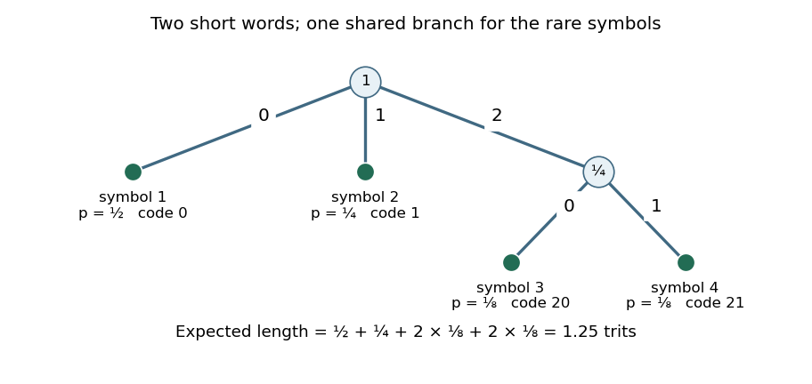

The shape of minimum-cost positive-weight ternary prefix trees arguments in ii–vi assume a full-support finite distribution: for every retained source symbol. The printed setup does not state this globally. Each affected solution gives the proof with that qualification and a counterexample when zero-probability symbols are allowed in arbitrary redundant code trees. Part i needs no such qualification.
Exchange the two complete codewords while leaving the code tree unchanged. The prefix code property is preserved because the set of codewords is unchanged. If but , the change in expected codeword length iscontradicting optimality. Hence implies . This probability monotonicity of optimal prefix-code lengths is valid even if some probabilities are zero; equal probabilities impose no order.[ref]
A Method for the Construction of Minimum-Redundancy Codes by David A. Huffman. p. 1099, Derived Coding Requirements: probability ordering and permissible exchange of equal-probability messages
First assume a full-support finite distribution, as stated above. Let be the largest codeword length and take a tree leaf at depth . Every existing tree child of its tree parent must also be a tree leaf: an internal tree child would have a descendant deeper than . If the chosen tree leaf were its tree parent's only tree child, moving its symbol to that tree parent would shorten its codeword by one, preserve the prefix code property, and reduce expected codeword length by its positive probability. That contradicts optimality. The tree parent therefore has at least two tree children, both tree leaves. A second codeword has the same first digits and a different last digit, proving the required deepest sibling codeword property for a ternary prefix code.
For the literal wording allowing zero probabilities, take and the prefix code . Its expected codeword length is one, which is minimal: with more than one message an empty codeword is impossible, so the positive-probability message must have length at least one. Yet the deepest tree leaf has no sibling codeword. Thus positivity or an additional convention removing redundant zero-weight branches is needed.
Articles were limited to the first 100 out of 1377 total.
Articles by others on the same topic
Year 3 of the mathematics course of the University of Oxford by  Ciro Santilli 40 Updated 2025-07-16