A mountain width is not an exactly specified sinusoidal wavelength. Taking its characteristic horizontal inverse length as with gives . Since , the stationary vertical wavenumber isThis is close to the long-horizontal-scale/hydrostatic estimate . If instead the quoted width is identified with a sinusoidal wavelength , then and . Thus several kilometres, roughly – under these two common width conventions, is the justified estimate; the terrain profile would fix its actual forcing spectrum.
For the inverse-width choice, both and are negative for upward energy radiation. The stationary phase lines tilt upstream with increasing height, while energy propagates upward and slightly downstream. Numerically , with ray inclination about . Intrinsic phase propagation points upstream and downwards; the ground pattern itself remains fixed. The original sketch below uses this explicit convention.
A ground observer may see stationary lenticular or wave clouds where ascent cools sufficiently moist air, with continuing air flow through a cloud whose position remains almost fixed. Descending regions can clear or warm. An aircraft crossing the pattern encounters alternating updraughts and downdraughts; gliders can exploit the lift. Strong amplitudes, shear or rotors may cause turbulence, but a linear gravity wave can also be smooth, and clear-air waves need not produce any visible cloud. Mountain height, humidity and nonlinear stability are not supplied, so neither a vertical-wind amplitude nor a definite atmospheric precipitation forecast follows.
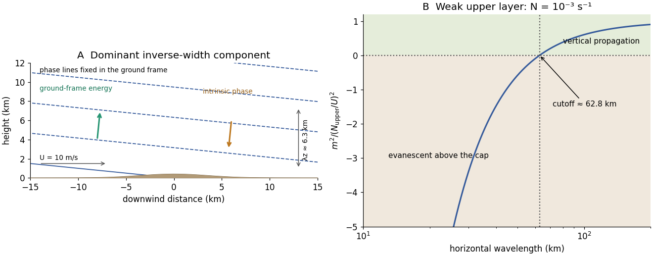
Stationary mountain-wave phase lines, intrinsic phase direction, energy rays and an upper-layer propagation cutoff
. Original schematic and dispersion calculation. The ridge height is illustrative; the phase sketch uses , while the upper-layer panel shows the cutoff for the reduced Brunt–Väisälä frequency. No cloud or turbulence amplitude is inferred. Details.
Articles by others on the same topic
There are currently no matching articles.