Let point to the equatorial meridian at zero longitude, to the equator at E, and to the north pole. Use a right-hand positive Euler angular velocity vector. Relative rotations add as vectors, not as geographic coordinates:ConsequentlyHere is the longitude of the positive Euler pole, and its latitude is zero. The antipodal pole with the opposite angular-velocity sign is an equivalent convention; mixing a pole reversal with an unchanged sign would give the wrong motion.
At latitude and longitude , . Motion is . A meridian boundary has horizontal normal , so its across-boundary velocity isFor a transform fault this must vanish along the whole meridian, not only at an isolated point. Thus . Select the solution in the western hemisphere:The other solution is the antipodal meridian in the eastern hemisphere. Geometrically, the transform meridian is in a great-circle plane perpendicular to the Euler angular velocity vector. Its outgoing tangent direction at either pole, expressed in the fixed axes, is .
At the south pole . Choose plate C as the instantaneous reference frame. Since mm, the two components of relative angular speed give 20 and 48 mm/year. The plate velocities in the fixed tangent-plane axes areThe plate velocity triangle therefore has sidesThe physical boundary rays point along for AB, for AC and for BC. Plate A occupies the quadrant between the first two rays, B the narrow wedge between AB and BC, and C the remainder. The stated overriding relations make AB and AC subduction trenches, while BC remains a transform fault: this is a trench-trench-transform triple junction. Put the subduction teeth on B's side of AB and A's side of AC, identifying B above A and A above C.
For kinematic stability there must be a single junction velocity compatible with all three boundary-normal motions. Use the standard idealization that each trench's normal velocity is that of its overriding plate, with no independent rollback. AB is parallel to , so . AC is parallel to , so . The transform requires to be parallel to , which is true for this intersection. HenceThe southern triple junction is instantaneously kinematically stable. It is stationary relative to B, migrates along AB relative to A, and migrates along BC relative to C. This compatibility result does not promise long-term stability if plate rotations or trench rollback change. Notice that the three relative velocities close even though the overriding order is not a statement that all three plates move toward one common stationary point.
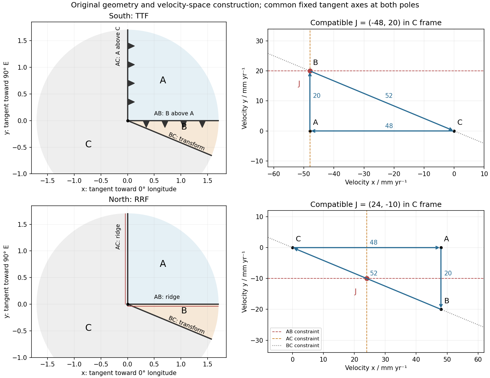
Original polar boundary geometry and plate velocity triangles; dashed velocity-space constraints locate compatible south and north junction velocities
. Details. 
At the north pole , so the velocities reverse:The triangle still has side lengths 20, 48 and 52 mm/year. Across AB, A moves toward positive relative to B; across AC, A moves toward positive relative to C. Both boundaries therefore open and are spreading ridges, with full opening speeds 20 and 48 mm/year. Together with BC they form a ridge-ridge-transform triple junction.
In the symmetric normal-spreading model, a ridge's normal velocity is the mean normal velocity of its two plates. AB gives , and AC gives . Their intersection lies on the BC transform velocity line:This northern junction is also instantaneously kinematically stable. The diagrams use the same fixed geocentric tangent axes at both poles; reversing velocities is not the same operation as reflecting a map drawn from an exterior observer's viewpoint.
Not every ridge-ridge-transform geometry works. For pure normal spreading, each ridge velocity line is the perpendicular bisector of the corresponding side of the plate velocity triangle. Their intersection is the triangle's circumcenter. A transform junction must also lie on the third side's line. A nondegenerate triangle's circumcenter lies there only at that side's midpoint, so the opposite angle is a right angle. Equivalently, . The two ridge directions are then perpendicular, as they are here. RRF junctions are conditionally stable, with the right-angle ridge geometry in this symmetric pure-normal model; they are not all stable. Oblique or asymmetric accretion changes the velocity-line assumptions and must be specified separately.
Assume an Earth-like reversing planetary magnetic field and magnetizable crust that acquires thermoremanent magnetization on cooling. Alternating polarity intervals then produce marine magnetic stripes parallel to each spreading ridge, with matching age/polarity sequences on its two sides. AB has half-spreading rate 10 mm/year, whereas AC has half-spreading rate 24 mm/year. Thus the same polarity interval produces widths and mm when time is in years: the AC stripes are 2.4 times wider. Age increases away from each ridge. The transform produces no new crust; bands end or are displaced at it, rather than forming a third symmetric stripe sequence centred on BC. This is the remanent-magnetization/spreading mechanism developed from marine magnetic observations.[ref]
Magnetic Anomalies Over Oceanic Ridges by F. J. Vine and D. H. Matthews. pp. 947–949, alternating remanent magnetization and the spreading interpretation
A more precise local sketch can be made in the northern junction frame. Let be distances in kilometres along the fixed tangent axes and the crustal age in Myr; numerically, mm/year equals km/Myr. Relative to the moving junction, the velocities are , and . In A the steady age field is , since backwards advection first reaches either the AC or AB ridge. Equal-age bands therefore join as right-angle corners within A, with the corners migrating along the ray . In the B wedge, and the stripes meet the transform. On the C flank directly supplied from AC, ; other parts of C carry older crust whose inherited pattern requires earlier boundary history.
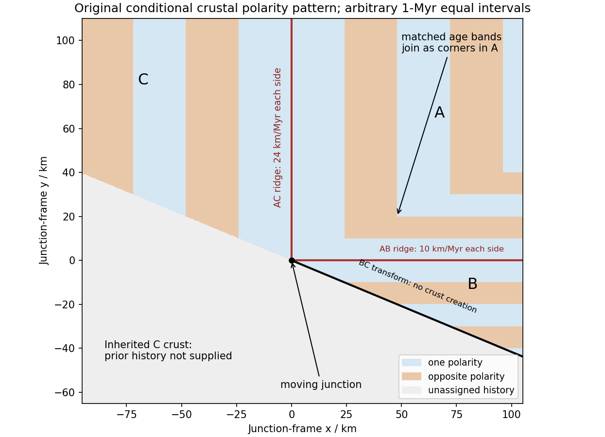
Original conditional remanent-polarity sketch in the north-junction frame; reversal intervals are illustrative and unsupplied older crust is left unassigned
. Details. 
The sketch displays magnetization polarity, not a computed total-field anomaly amplitude. Actual anomalies depend on the planetary field direction, source depth, magnetization strength and observation geometry. The paper supplies no field history, so a numerical reversal chronology or an absolute positive/negative anomaly sequence cannot be inferred. Without field reversals, ridge accretion alone does not imply alternating polarity stripes.
Articles by others on the same topic
There are currently no matching articles.