Original solutions to the released 2016 1/PEP paper. [ref]
https://www.whatdotheyknow.com/request/natural_science_tripos_physics_e_2/response/2340776/attach/2/FOI%202023%20399%20Zahid%20materials.pdf?cookie_passthrough=1#page=790. Original public PDF, physical pages 790–793; questions on pages 791–793
Let point to the equatorial meridian at zero longitude, to the equator at E, and to the north pole. Use a right-hand positive Euler angular velocity vector. Relative rotations add as vectors, not as geographic coordinates:ConsequentlyHere is the longitude of the positive Euler pole, and its latitude is zero. The antipodal pole with the opposite angular-velocity sign is an equivalent convention; mixing a pole reversal with an unchanged sign would give the wrong motion.
At latitude and longitude , . Motion is . A meridian boundary has horizontal normal , so its across-boundary velocity isFor a transform fault this must vanish along the whole meridian, not only at an isolated point. Thus . Select the solution in the western hemisphere:The other solution is the antipodal meridian in the eastern hemisphere. Geometrically, the transform meridian is in a great-circle plane perpendicular to the Euler angular velocity vector. Its outgoing tangent direction at either pole, expressed in the fixed axes, is .
At the south pole . Choose plate C as the instantaneous reference frame. Since mm, the two components of relative angular speed give 20 and 48 mm/year. The plate velocities in the fixed tangent-plane axes areThe plate velocity triangle therefore has sidesThe physical boundary rays point along for AB, for AC and for BC. Plate A occupies the quadrant between the first two rays, B the narrow wedge between AB and BC, and C the remainder. The stated overriding relations make AB and AC subduction trenches, while BC remains a transform fault: this is a trench-trench-transform triple junction. Put the subduction teeth on B's side of AB and A's side of AC, identifying B above A and A above C.
For kinematic stability there must be a single junction velocity compatible with all three boundary-normal motions. Use the standard idealization that each trench's normal velocity is that of its overriding plate, with no independent rollback. AB is parallel to , so . AC is parallel to , so . The transform requires to be parallel to , which is true for this intersection. HenceThe southern triple junction is instantaneously kinematically stable. It is stationary relative to B, migrates along AB relative to A, and migrates along BC relative to C. This compatibility result does not promise long-term stability if plate rotations or trench rollback change. Notice that the three relative velocities close even though the overriding order is not a statement that all three plates move toward one common stationary point.
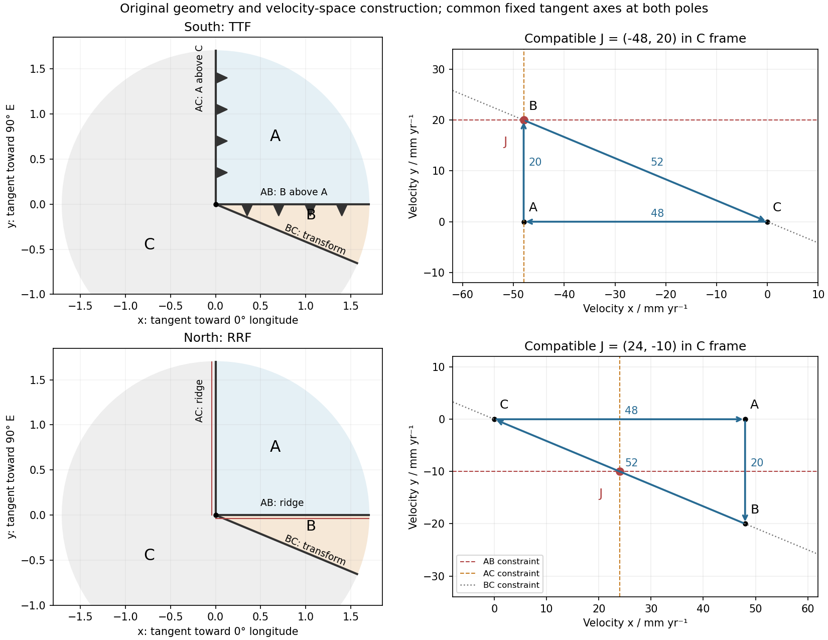
Original polar boundary geometry and plate velocity triangles; dashed velocity-space constraints locate compatible south and north junction velocities
. Details. 
At the north pole , so the velocities reverse:The triangle still has side lengths 20, 48 and 52 mm/year. Across AB, A moves toward positive relative to B; across AC, A moves toward positive relative to C. Both boundaries therefore open and are spreading ridges, with full opening speeds 20 and 48 mm/year. Together with BC they form a ridge-ridge-transform triple junction.
In the symmetric normal-spreading model, a ridge's normal velocity is the mean normal velocity of its two plates. AB gives , and AC gives . Their intersection lies on the BC transform velocity line:This northern junction is also instantaneously kinematically stable. The diagrams use the same fixed geocentric tangent axes at both poles; reversing velocities is not the same operation as reflecting a map drawn from an exterior observer's viewpoint.
Not every ridge-ridge-transform geometry works. For pure normal spreading, each ridge velocity line is the perpendicular bisector of the corresponding side of the plate velocity triangle. Their intersection is the triangle's circumcenter. A transform junction must also lie on the third side's line. A nondegenerate triangle's circumcenter lies there only at that side's midpoint, so the opposite angle is a right angle. Equivalently, . The two ridge directions are then perpendicular, as they are here. RRF junctions are conditionally stable, with the right-angle ridge geometry in this symmetric pure-normal model; they are not all stable. Oblique or asymmetric accretion changes the velocity-line assumptions and must be specified separately.
Assume an Earth-like reversing planetary magnetic field and magnetizable crust that acquires thermoremanent magnetization on cooling. Alternating polarity intervals then produce marine magnetic stripes parallel to each spreading ridge, with matching age/polarity sequences on its two sides. AB has half-spreading rate 10 mm/year, whereas AC has half-spreading rate 24 mm/year. Thus the same polarity interval produces widths and mm when time is in years: the AC stripes are 2.4 times wider. Age increases away from each ridge. The transform produces no new crust; bands end or are displaced at it, rather than forming a third symmetric stripe sequence centred on BC. This is the remanent-magnetization/spreading mechanism developed from marine magnetic observations.[ref]
Magnetic Anomalies Over Oceanic Ridges by F. J. Vine and D. H. Matthews. pp. 947–949, alternating remanent magnetization and the spreading interpretation
A more precise local sketch can be made in the northern junction frame. Let be distances in kilometres along the fixed tangent axes and the crustal age in Myr; numerically, mm/year equals km/Myr. Relative to the moving junction, the velocities are , and . In A the steady age field is , since backwards advection first reaches either the AC or AB ridge. Equal-age bands therefore join as right-angle corners within A, with the corners migrating along the ray . In the B wedge, and the stripes meet the transform. On the C flank directly supplied from AC, ; other parts of C carry older crust whose inherited pattern requires earlier boundary history.
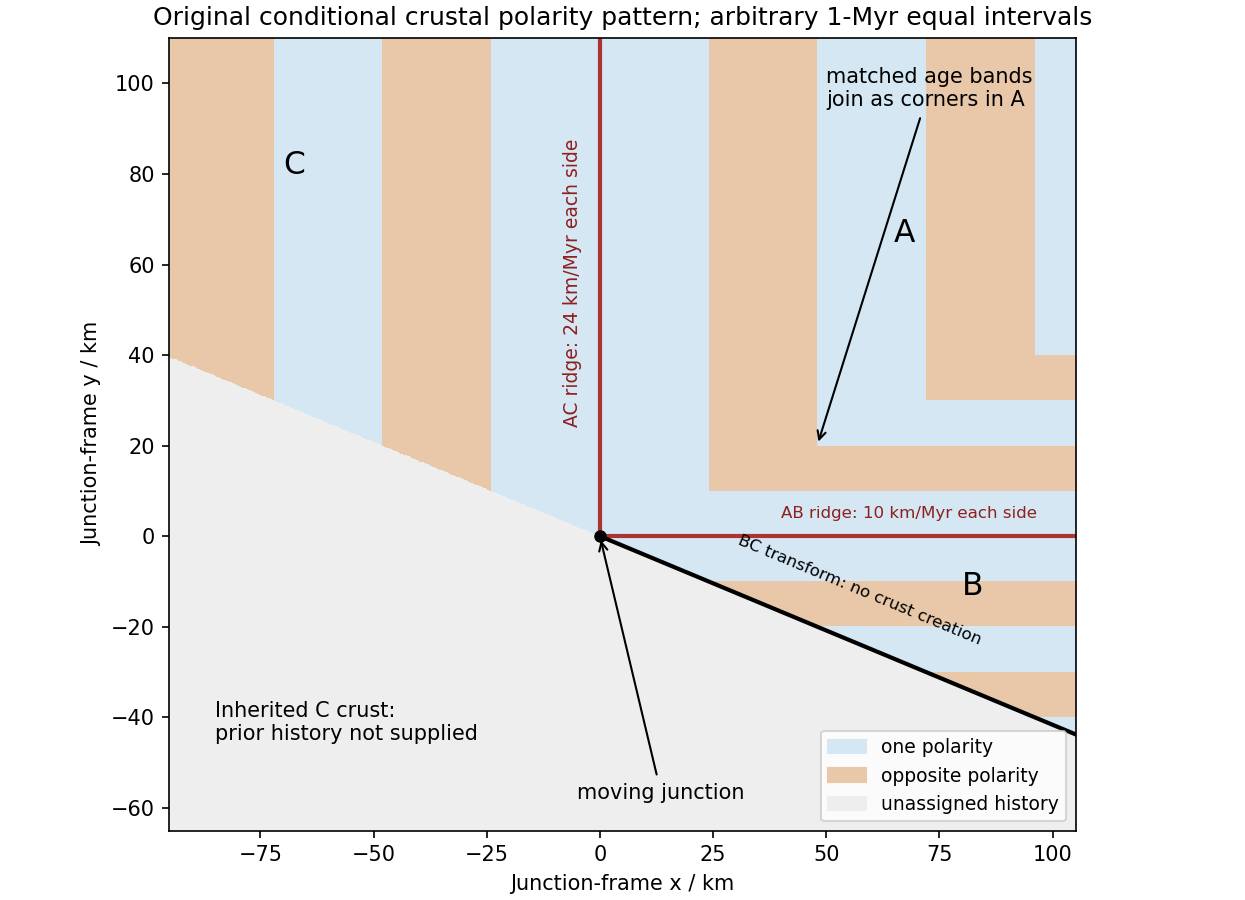
Original conditional remanent-polarity sketch in the north-junction frame; reversal intervals are illustrative and unsupplied older crust is left unassigned
. Details. 
The sketch displays magnetization polarity, not a computed total-field anomaly amplitude. Actual anomalies depend on the planetary field direction, source depth, magnetization strength and observation geometry. The paper supplies no field history, so a numerical reversal chronology or an absolute positive/negative anomaly sequence cannot be inferred. Without field reversals, ridge accretion alone does not imply alternating polarity stripes.
gravity and surface topography. gravity responds to all density structure, while surface topography records both load and support. First specify the reference field and measurement height. latitude and planetary rotation affect normal gravity. At elevation , the reference field decreases approximately by ; a free-air gravity anomaly restores this elevation effect but retains topographic mass. A Bouguer gravity anomaly additionally subtracts an approximate topographic slab contribution . terrain correction replaces the unrealistic slab near valleys and ridges, and spherical geometry matters over large areas. A density choice is required for these reductions; a numerical crustal density is not provided here.
In Airy isostasy, surface topography of height and crustal density is compensated by a root of thickness replacing mantle of density . Equal column masses give . The positive gravity of the relief is partly cancelled by the negative density contrast of the root. At long wavelengths a compensated mountain can therefore have a modest free-air anomaly and a negative Bouguer anomaly. Pratt isostasy instead varies column density at a roughly common compensation depth. Neither model says that surface topography itself exerts no gravity.
Potential-field depth filtering makes wavelength crucial. In a planar Fourier approximation, a density interface at depth is attenuated by at horizontal wavenumber . For a small Airy-compensated height perturbation and a compensation interface at depth , the gravity-topography admittance is approximatelyLong wavelengths allow strong cancellation between load and root. At short wavelengths the root's gravity is filtered out, so the observed near-surface mass can dominate even if the column is compensated. In a flexural isostasy model, an elastic lithosphere supports and spreads the load; for downward deflection and imposed load , , with . Thus , and the effective elastic thickness controls the support scale.
Estimate admittance from cross-spectra of gravity and surface topography, and compare its wavelength dependence and coherence with local-compensation, elastic-flexure and subsurface-load models. A primary Atlantic study sampled ship-track free-air gravity and bathymetry and compared their Fourier-domain relationship with compensation models, illustrating this observational route rather than inferring a root from the sign of one gravity value.[ref]
The relationship between bathymetry and gravity in the Atlantic Ocean by Dan McKenzie and Carl Bowin. pp. 1903–1915, ship-track sampling, spectral transfer estimates and wavelength-dependent compensation
Check navigation, instrument drift, terrain/density reductions, sediment and water loads, and independent seismic crustal constraints. Density-depth trade-offs and mantle dynamic support make the inverse problem nonunique; surface topography and gravity together constrain support, but do not uniquely map every density anomaly.mantle viscosity. A second, independent route concerns deformation rates rather than static compensation. glacial isostatic adjustment follows loading and unloading of a deformable Earth: an ice sheet depresses the surface, and subsequent removal leaves time-dependent uplift, horizontal displacement, sea-level and gravity changes. Fit dated relative sea-level indicators and raised shorelines together with geodetic displacement rates and a reconstructed ice/water load history to a viscoelastic Earth model. Relative sea level includes solid-surface motion, changing geoid and redistribution of ocean water; treating it only as local vertical rock motion biases the inference.
For scale, a sinusoidal surface perturbation of wavenumber on a uniform incompressible viscous half-space relaxes under gravity with . A Maxwell material separately has a stress-relaxation scale . These are different experiments and generally different times: rebound modes also involve gravity, spherical geometry, a layered mantle and elastic lithosphere. Fit a family of relaxation modes or a full load-history convolution, rather than equating every observed rebound time to .
Use independent ice-margin, exposure-age and sea-level constraints to reduce the trade-off between ice history and viscosity; compare horizontal as well as vertical GNSS motions, and separate present ice loss, groundwater changes and tectonic signals from the older loading response. A primary global analysis jointly tested ice-history and mantle-response predictions against space-geodetic observations, rather than treating a local uplift rate as a unique viscosity measurement.[ref]
postseismic relaxation probes shallower or faster relaxation after a stress perturbation, but must be distinguished from afterslip and poroelastic deformation. Long-wavelength geoid and mantle-flow models provide complementary constraints when density structure is estimated independently from seismic structure and mineral physics; unknown density-to-velocity conversion and boundary tractions remain trade-offs. Laboratory creep experiments constrain constitutive laws as functions of temperature, stress and grain size, but require a large extrapolation to geological conditions. Combine spatially and temporally distinct observations; there is no single directly measured mantle viscosity independent of depth, rheology and loading assumptions.
First-motion source mechanisms. Locate an earthquake from arrival times and use a seismic velocity model to calculate each station's source takeoff direction. Measure the initial direct P wave polarity after checking instrument sign, component orientation, timing and phase identification. An upward trace at an instrument is not automatically a source compression without the propagation and component convention. Plot the inferred source radiation signs on a focal sphere, commonly using a lower-hemisphere equal-area projection, and seek nodal planes separating positive and negative observations.
For a shear dislocation with orthogonal unit slip and fault-normal vectors , the double-couple fault source has . Its far-field P radiation sign is that ofThe two zeros are orthogonal nodal planes; the four quadrants alternate between outward and inward initial radiation. Their orientations and quadrant signs determine candidate strike, dip and rake. Normal, reverse and strike-slip mechanisms give different projected patterns. The earthquake pressure and tension axes are the negative and positive moment-tensor principal directions, respectively; they do not by themselves measure the complete regional stress tensor.
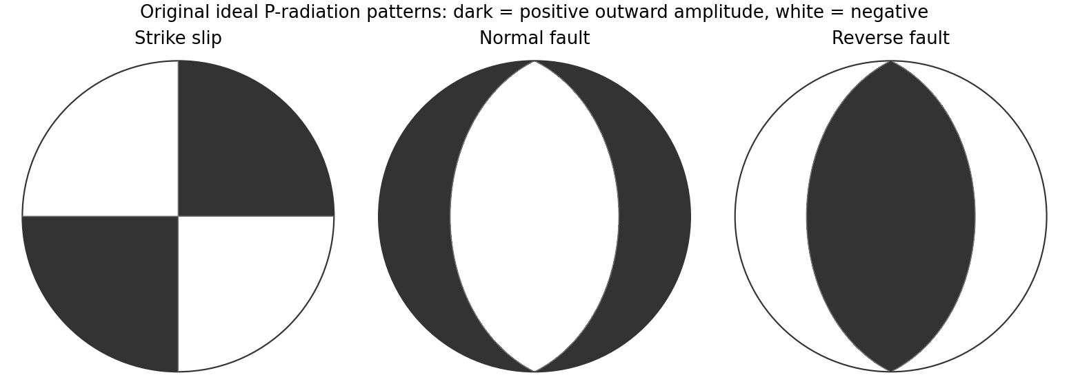
Original lower-hemisphere equal-area P-radiation polarity examples for ideal strike-slip, normal and reverse double couples
. Details. 
There is a fundamental fault-plane ambiguity: exchanging and leaves the radiation tensor unchanged. First motions therefore give a fault plane and an auxiliary plane without saying which actually slipped. Use mapped rupture, aftershock geometry or independent geodetic displacement to select the physical fault where possible. Polarity signs alone do not measure scalar seismic moment, source duration or rupture extent. A poorly sampled focal sphere or many near-nodal observations can admit several mechanisms rather than one defensible beachball.
Propagate uncertainty in event depth, velocity gradients and takeoff angles, allow for mispicked or reversed polarities, and report the range of mechanisms consistent with the observations. A primary method did this by testing alternative locations and velocity models and validated its uncertainty estimates using noisy synthetic data and clusters of events with similar waveforms.[ref]
A New Method for Determining First-Motion Focal Mechanisms by Jeanne L. Hardebeck and Peter M. Shearer. pp. 2264–2266 and abstract, first-motion construction, polarity/takeoff uncertainty and independent validation tests
Broadband waveforms and amplitude ratios add information, especially for non-double-couple sources, but they are additional measurements rather than a way to extract amplitude information from a sign-only data set.Radial density structure. In an isotropic adiabatic material, the seismic parameter isFor a chemically homogeneous region whose background stratification is adiabatic, . Combine this with spherical hydrostatic balance and mass conservation to obtain the Adams-Williamson equationsThe inward density increase follows compressibility under the increasing pressure. A specified starting density and measured allow integration within a homogeneous adiabatic layer. Seismic velocities alone, however, do not determine that density normalization, since they contain ratios of moduli to density. Chemical boundaries, phase transitions, nonadiabatic thermal gradients and anisotropy require additional modeling; a composition jump is not obtained by blindly integrating the smooth relation across it.
Use travel times and surface waves to constrain elastic velocities, reflected/converted phases to locate interfaces, and normal-mode frequencies to constrain density as well as elastic structure through their sensitivity kernels. Impose independently known total mass and moment of inertia:Because these weight depth differently, they help distinguish admissible profiles, but two integrals alone do not specify an arbitrary radial function. Laboratory equations of state and mineral physics restrict composition, compressibility and density jumps. pressure and enclosed mass are matched across interfaces, while density may jump. In a liquid region and , so the shear-wave absence constrains phase state without itself providing a direct density measurement.
The Preliminary Reference Earth Model is a concrete joint inversion of seismic travel times, normal modes, mass and inertia, including density and attenuation along with elastic structure. The original analysis combined these complementary data rather than deriving density uniquely from P wave speed.[ref]
Preliminary reference Earth model by Adam M. Dziewonski and Don L. Anderson. abstract and pp. 297–300, data classes and coupled radial reference-model inversion
A defensible radial density model combines hydrostatic/thermodynamic relations with seismic and global integral constraints, and states where homogeneity and adiabaticity fail.For uniform density and stiffness, linear momentum balance without body force is . The minor elastic symmetries make the two symmetric-strain terms equal, so . Write and . Then and . Thus a nontrivial plane-wave profile satisfiesThe density-normalized elastic acoustic tensor is consequentlyThe alternative dummy-index form is identical. In ordinary conservative elasticity, major symmetry gives after interchanging the dummy indices. This symmetry comes from a strain-energy density; it is an assumption of the ordinary elastic tensor, not a consequence of homogeneity alone.
For any such eigenpair the profile is arbitrary, since both sides carry the same . This nondispersive result uses linear, local, time-independent elasticity without attenuation or spatial dispersion. A profile with is a trivial uniform or affine displacement field and cannot be used by itself to infer the wave-speed eigenvalue condition.
A real symmetric matrix has three real eigenvalues and a complete orthonormal basis of eigenvectors. For a stable elastic material, strong ellipticity makes for every nonzero polarization, so its eigenvalues are positive squared wave speeds. There are therefore three orthogonal plane-wave polarizations in a given direction, with three potentially distinct speeds in an anisotropic medium. Degenerate eigenvalues allow arbitrary orthonormal combinations within their eigenspace; they do not remove polarization degrees of freedom. General anisotropic modes need not be exactly longitudinal or transverse.
For an isotropic medium let . Contract the isotropic stiffness with :UsinggivesFor the longitudinal projector has eigenvalue one, so : this is the P wave. For either of two independent the projector vanishes, so : these are two degenerate transverse S wave polarizations. An isotropic solid has one P speed and one S speed, but three polarization modes: one longitudinal and two transverse. A fluid limit with zero shear modulus has no propagating S wave, so the positive-speed conclusion requires a solid with positive shear stiffness.
Use geometric rays for body-wave arrivals and a traction-free upper surface. A compact isotropic explosion source has moment tensor proportional to and produces direct P body radiation in a homogeneous isotropic medium. Thus the basic near-offset arrival is the direct upper-layer P wave, with time . A pure explosion is not a shear fault: it does not automatically emit a direct S wave of comparable strength. Interfaces can nevertheless convert its P energy into SV motion, and the free surface can support Rayleigh waves.
Downward P energy reflects from the interface to give a PP reflection returning to the receiver; for a horizontal interface its ray is symmetric and its time is . Other transmitted P energy enters the faster half-space. At , a critical ray travels along the interface and feeds an upgoing seismic head wave, often labeled Pn in this simplified crustal model. Its ideal travel-time branch isIt requires enough offset for the two inclined upper-layer legs, . Once exceeds the larger first-arrival crossover distance , this branch arrives before the direct upper-layer wave because it spends most of the path in faster material. A transmitted ray descending into an otherwise uniform infinite half-space does not return as a separate reflection without an additional reflector.
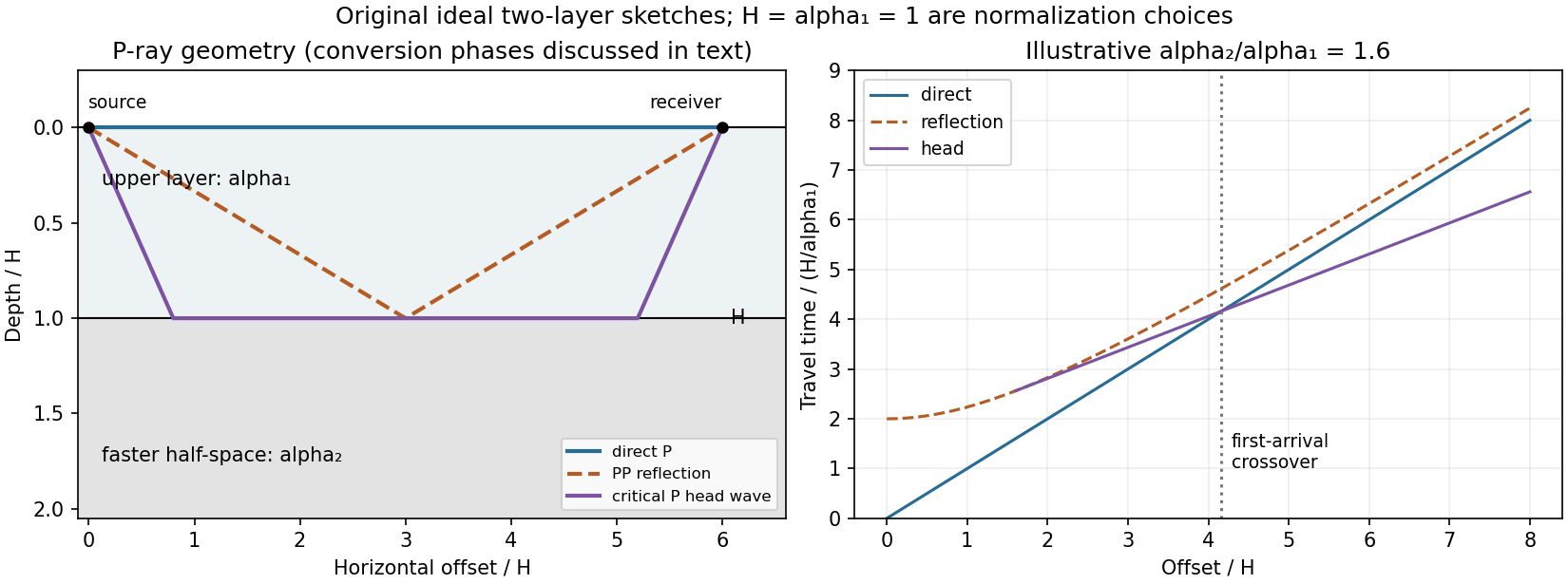
Original two-layer P-ray sketches and illustrative direct, reflected and critically refracted travel-time branches
. Details. 
At oblique incidence, the bonded-interface conditions couple P and SV polarizations. A downgoing P ray can return as a converted SV reflection in the upper layer, with common horizontal slowness . There are transmitted P/SV branches and, after further interaction with the free surface or interface, mixed-mode reflections and layer reverberations. Conversion coefficients depend on density and impedance as well as wave speeds, and some vanish at normal incidence. The supplied inequalities do not order against , so one cannot universally draw a P-incident critical head ray travelling at the lower-layer S speed: that direct conversion construction requires . A shear head-wave phase can be present if the appropriate SV energy and ray conditions are available, but is not an inevitable direct explosion arrival from the stated data alone.
At later times a shallow explosion can excite dispersive Rayleigh-wave trains, with coupled P-SV motion decaying with depth. Short wavelengths mainly sample the slow upper layer, whereas long wavelengths penetrate the lower half-space; group and phase speeds need not be equal. Multiple reflected/converted body waves can overlap this coda. The shear-speed contrast also permits Love-wave modes structurally, but SH motion is decoupled from P-SV in this flat isotropic model. An ideal isotropic explosion does not excite Love waves here; appreciable SH/Love energy would require source asymmetry, scattering or a broken symmetry of the model.
Exact amplitudes, resolved arrival separation and attenuation cannot be calculated without densities, source spectrum, damping and instrument response. The qualitative robust features are a near-offset direct P arrival, reflected and converted phases, a faster-lower-layer P head wave that can become first at long range, reverberations and P-SV surface-wave energy. The ray diagram uses declared illustrative speed ratios solely to show the geometry; they are not additional supplied material constants.
Articles by others on the same topic
There are currently no matching articles.