Past exam of the topics in applied mathematics course of the University of Oxford / 2008 / A / 1

Write $P(N)=f(N,0)$. Its three positive zeros of a function are $1/2,1,2$, and expansion and differentiation giveThus its local minimum and maximum occur respectively atwith valuesThe function graph approaches the value $1$ as $N\downarrow 0$, decreases through its first zero to the minimum, increases through its second zero to the maximum, and then decreases through $2$ to $-\infty$. This fixes the shape and all axis crossings of the cubic polynomial.

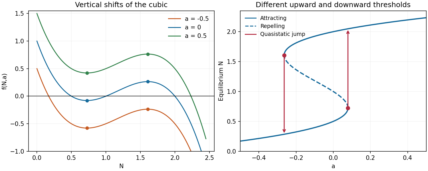
Changing $a$ translates the function graph vertically without moving either stationary point. For $a=1/2$ both extrema are above the horizontal axis: their heights are approximately $0.421109$ and $0.764076$. For $a=-1/2$ both are below it, at approximately $-0.578891$ and $-0.235924$. The function graph for $a=1/2$ therefore has only its final positive-axis crossing, whereas the function graph for $a=-1/2$ has only its first positive-axis crossing. The original plots mark the extrema and also show the equilibrium point branches used below.

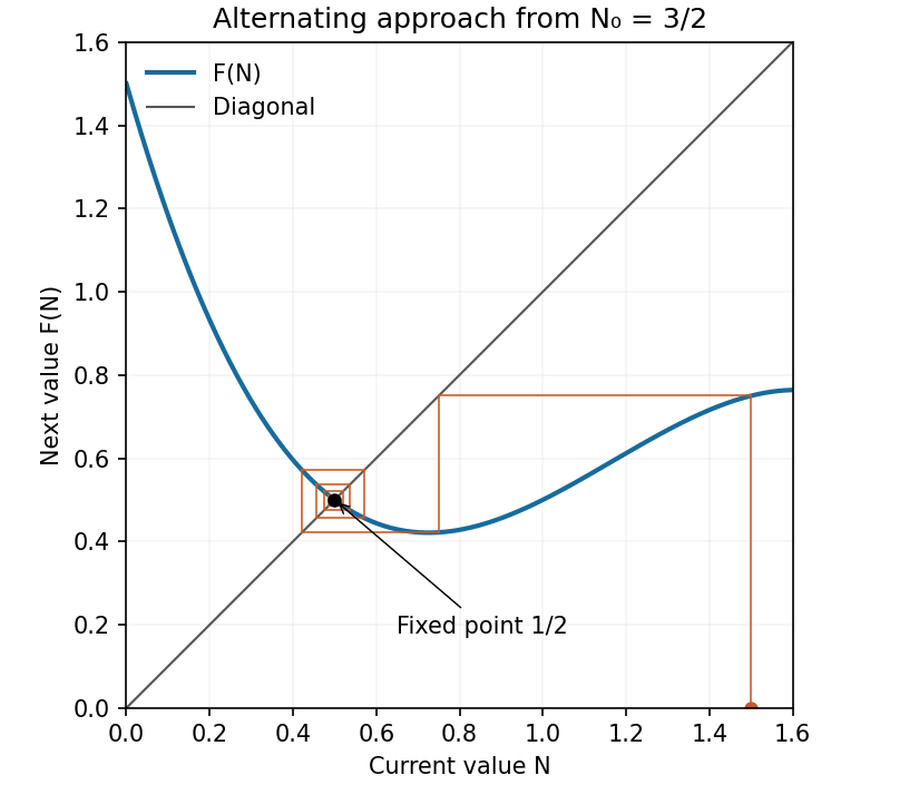
Put $F(N)=f(N,1/2)$. A cobweb plot alternates a vertical move to the function graph $y=F(N)$ with a horizontal move to the diagonal $y=N$. Beginning at $N_0=3/2$, the first iterates areThe diagram shows the ensuing approach to $1/2$ with alternating deviations. More precisely, if $e_t=N_t-1/2$, Taylor expansion at the fixed point givesFor sufficiently small nonzero deviations the sign reverses each step and their magnitudes contract. The local approach is an alternating, geometrically damped oscillation, with asymptotic contraction factor $3/4$ per iterate.

First establish a uniform upper bound. Direct subtraction givesbecause the quadratic polynomial has positive leading coefficient and discriminant $49-56=-7$. The assumed positivity of $F(N_0)$ therefore places $N_1$ in $(0,3/2)$.

This interval is forward invariant. On $[0,1/2]$ and on $[1,3/2]$, the three factors in $P(N)$ have nonnegative product, hence $F(N)\ge 1/2$. On $[1/2,1]$ the product is nonpositive, butso $F(N)\ge 1/8>0$. Together with the upper bound this proves $F((0,3/2))\subset (0,3/2)$. Induction now givesThe hypothesis on the first image is essential for initial values outside that invariant interval.

For an autonomous scalar differential equation, linear stability of a simple equilibrium point $N_e$ is determined by the derivative $f_N(N_e,a)=P^{\prime }(N_e)$: a negative derivative attracts nearby solutions and a positive derivative gives repulsion in a dynamical system of nearby solutions.

Here $f(0,a)=1+a\ge 1/2>0$ throughout the prescribed mathematical model parameter range, while $f(N,a)\to -\infty$ as $N\to \infty$. If there is only one equilibrium point, the function graph must cross the axis on one of its decreasing branches, outside the interval between its two extrema. The crossing is simple and $P^{\prime }(N_e)<0$. Thus the unique equilibrium point is linearly asymptotically stable. At a saddle-node bifurcation there are two distinct equilibrium points, one of them double, so that case does not fall under the one-equilibrium hypothesis.

With three distinct positive roots of an equation, the negative-leading cubic polynomial has the sign patternEquivalently its derivative is negative at the first root of an equation, positive at the middle root of an equation, and negative at the final root of an equation. The phase line arrows therefore point toward the two outer equilibrium points and away from the middle one:The middle equilibrium point separates the two basin of attraction in the bistability mathematical model parameter interval.

Yes: there is a quasistatic hysteresis loop. Equilibrium points lie on the mathematical model parameter curve $a=-P(N)$. Its two saddle-node bifurcations occur at the stationary points computed in part (a), at mathematical model parameter valuesBetween these values there are two attracting branches separated by a repelling branch. Starting below $a_{\mathrm{down}}$ and increasing $a$ slowly, a solution follows the lower attracting branch. This branch persists through the bistability interval and ends only at $a_{\mathrm{up}}$, where it meets the repelling branch in a saddle-node bifurcation. The solution then moves to the upper attracting branch.

If the direction of mathematical model parameter change is reversed, the upper branch persists until $a_{\mathrm{down}}$, where a different saddle-node bifurcation forces the downward transition. The two transition values differ, and both lie inside the allowed range $[-1/2,1/2]$. Thus the biological population selected at an intermediate mathematical model parameter value depends on its prior branch. This is the equilibrium point hysteresis shown in the branch diagram; finite-rate passage can additionally delay the jumps near the saddle-node bifurcations.