This University of Oxford Part B paper is cross-listed for Mathematics and Mathematics and Statistics. Section A concerns mathematical biology, and section B concerns dynamical systems. [ref]
https://www.whatdotheyknow.com/request/maths_past_papers_3. Source release
The archive contains the complete editable eight-page transcription. Bounded searches of official sources found no advertised answers to this exact paper. The original solutions cover every source leaf and every unnumbered task in questions 5–8.Write . Its three positive zeros of a function are , and expansion and differentiation giveThus its local minimum and maximum occur respectively atwith valuesThe function graph approaches the value as , decreases through its first zero to the minimum, increases through its second zero to the maximum, and then decreases through to . This fixes the shape and all axis crossings of the cubic polynomial.
Changing translates the function graph vertically without moving either stationary point. For both extrema are above the horizontal axis: their heights are approximately and . For both are below it, at approximately and . The function graph for therefore has only its final positive-axis crossing, whereas the function graph for has only its first positive-axis crossing. The original plots mark the extrema and also show the equilibrium point branches used below.
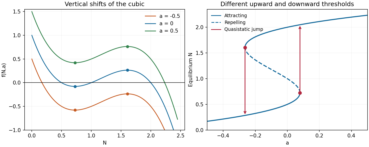
Cubic graphs and equilibrium branches
. Details. Put . A cobweb plot alternates a vertical move to the function graph with a horizontal move to the diagonal . Beginning at , the first iterates areThe diagram shows the ensuing approach to with alternating deviations. More precisely, if , Taylor expansion at the fixed point givesFor sufficiently small nonzero deviations the sign reverses each step and their magnitudes contract. The local approach is an alternating, geometrically damped oscillation, with asymptotic contraction factor per iterate.
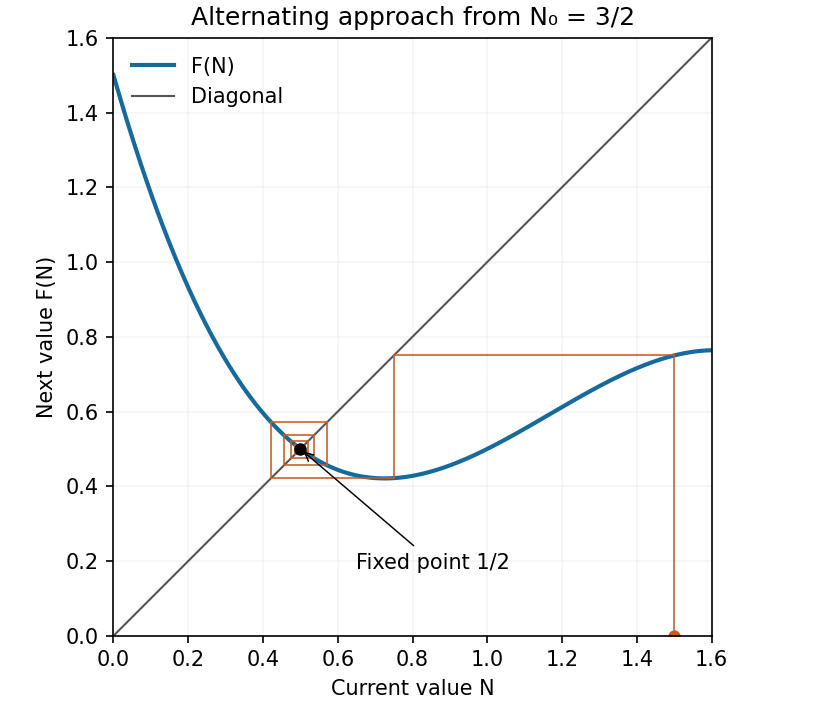
Cobweb approaching the attracting fixed point
. Details. First establish a uniform upper bound. Direct subtraction givesbecause the quadratic polynomial has positive leading coefficient and discriminant . The assumed positivity of therefore places in .
This interval is forward invariant. On and on , the three factors in have nonnegative product, hence . On the product is nonpositive, butso . Together with the upper bound this proves . Induction now givesThe hypothesis on the first image is essential for initial values outside that invariant interval.
For an autonomous scalar differential equation, linear stability of a simple equilibrium point is determined by the derivative : a negative derivative attracts nearby solutions and a positive derivative gives repulsion in a dynamical system of nearby solutions.
Here throughout the prescribed mathematical model parameter range, while as . If there is only one equilibrium point, the function graph must cross the axis on one of its decreasing branches, outside the interval between its two extrema. The crossing is simple and . Thus the unique equilibrium point is linearly asymptotically stable. At a saddle-node bifurcation there are two distinct equilibrium points, one of them double, so that case does not fall under the one-equilibrium hypothesis.
With three distinct positive roots of an equation, the negative-leading cubic polynomial has the sign patternEquivalently its derivative is negative at the first root of an equation, positive at the middle root of an equation, and negative at the final root of an equation. The phase line arrows therefore point toward the two outer equilibrium points and away from the middle one:The middle equilibrium point separates the two basin of attraction in the bistability mathematical model parameter interval.
Yes: there is a quasistatic hysteresis loop. Equilibrium points lie on the mathematical model parameter curve . Its two saddle-node bifurcations occur at the stationary points computed in part (a), at mathematical model parameter valuesBetween these values there are two attracting branches separated by a repelling branch. Starting below and increasing slowly, a solution follows the lower attracting branch. This branch persists through the bistability interval and ends only at , where it meets the repelling branch in a saddle-node bifurcation. The solution then moves to the upper attracting branch.
If the direction of mathematical model parameter change is reversed, the upper branch persists until , where a different saddle-node bifurcation forces the downward transition. The two transition values differ, and both lie inside the allowed range . Thus the biological population selected at an intermediate mathematical model parameter value depends on its prior branch. This is the equilibrium point hysteresis shown in the branch diagram; finite-rate passage can additionally delay the jumps near the saddle-node bifurcations.
The term is a mass-action incidence rate: each infective individual makes potentially transmitting contacts with susceptible individuals, and the total rate is proportional to the product of the two compartment sizes. An infection transfers one animal from to , accounting for opposite signs in their equations. The per-capita mortality rate of an infective individual is , giving transfer from to .
There are no births, recoveries or additional deaths in this model. Adding the three equations gives , so the total initial biological population is conserved when the dead compartment is included. Before quarantine, decreases whenever ; after effective isolation no further transmission is permitted.
Write and . Until quarantine and while , division of the equations givesIntegration from the initial state yields the first integralLet be the susceptible count at the first time . It is the root of an equation reached on the decreasing- outbreak trajectory ofFor a strictly rising threshold crossing this is the larger admissible root of an equation, with ; if the threshold equals the peak, . The assumption that quarantine is reached selects the physically relevant branch and excludes a merely hypothetical declining-branch crossing after an earlier one.
Since there is no incubation period here, all removals from have already become infection cases by quarantine. No further susceptible individuals are infected after isolation. The requested number among the initially susceptible individuals is therefore
The delayed influx represents animals exposed one incubation period earlier who enter the infective individual compartment now. They die at the instantaneous rate once in that compartment. The displayed bookkeeping removes an animal from at the same delayed time that it enters , preserving .
For this bookkeeping, must include the exposed animals which have not yet completed incubation period. If were instead defined as strictly unexposed susceptible individuals, its loss term would be the current exposure rate and a separate latent compartment would be needed. The calculations here follow the printed delay differential equation. A full initial-value problem for a delay differential equation also needs a history on ; the following small-delay expansion of an epidemic transfer rate concerns a smooth compatible history and the regular regime assumed by the question.
In the first-order Taylor expansion correction it suffices to use the zeroth-order derivatives. They giveThe delayed product is consequentlyMultiplying by and substituting into the two transfer equations producesThe opposite signs of and are also required by conservation law of : this correction changes the timing of the transfer between and , while leaving the instantaneous death term unchanged.
At the retained order define . Neglecting terms of order in the incidence correction givesDividing and expanding consistently,Thus the susceptible count at the first threshold crossing obeys the same retained-order equation as before:It is important to distinguish completed case transfers at quarantine from all infections already initiated. Let the quarantine time be . Isolation prevents exposures after , but animals exposed during still finish their incubation period during . Their number, in the printed bookkeeping, isThe infection cases transferred by time among the initial class number . Adding those pending infection cases gives the eventual number who catch the infectious disease:This adds only infections caused by exposures before isolation; it does not allow secondary transmission after quarantine. If one asks instead only for the transfers completed by the instant of quarantine, the answer is . The distinction is necessary because the model keeps incubating animals in its compartment.
An unbiased random walk of bacteria leads, on the continuum scale, to diffusion with coefficient , represented by . The cell proliferation rate is proportional both to the available biological growth factor concentration and to the bacterial density. Consumption of biological growth factor at rate gives its negative reaction term.
There is no diffusion term for because the biological growth factor is attached to the substrate rather than freely transported. There is also no chemotactic drift in this model: the specified motion is random, while the biological growth factor changes cell proliferation rather than directional movement. Both reaction terms vanish if either bacteria or biological growth factor are absent.
Choose a positive reference biological growth factor concentration , for example its concentration ahead of the travelling wave. SetwhereThe chain rule then transforms the equations intoEach displayed coefficient is one with the chosen scales. Hence the dimensionless system isThe free choice of expresses the freedom to normalize the as-yet unspecified concentration scale.
Take profiles and with , and use a prime for differentiation with respect to . The chain rule gives , and . ThereforeThese are coupled ordinary differential equations for a right-moving travelling wave with speed . A first-order formulation, using , is , , . In particular a positive profile has , consistent with depleted substrate behind the travelling front and fresh biological growth factor ahead.
Substitute into the bacterial profile equation. This giveswhich integrates once toAt the asymptotic constant states the profile derivative tends to zero. The state ahead of the travelling wave, where and , therefore gives . The state behind it, where and , gives . Since ,This first integral expresses the matching between biomass produced and biological growth factor consumed after the chosen nondimensionalization.
At the leading edge and . The linearized bacterial equation iswith characteristic exponentsFor they form a nonreal complex conjugate pair. A nonzero profile approaching the travelling front then has an exponentially decaying oscillatory leading term, and repeatedly changes sign. This is incompatible with the assumed positive bacterial density. The leading edge must therefore have real characteristic exponents, requiringAt the repeated characteristic exponent is and polynomial factors in the asymptotic profile may occur. The argument supplies a necessary lower bound; it is not an independent existence proof for every speed satisfying it.
The first integral and yield the linear identity . Multiply by the integrating factor and integrate from . Since the bounded limit makes there,Positivity of makes the last integral nonnegative, and strictly positive at any finite point of a strictly positive travelling wave. Thuswith equality approached only at the far-behind boundary. This bound uses the first integral rather than an unsupported assumption that the bacterial profile is monotone.
For the modified strain the travelling wave equations areIntegrating the second across the entire travelling wave gives , since the biological growth factor profile still goes from to . Integrating the first, using the constant asymptotic states and vanishing derivative at infinity, givesConsequentlyThe subtracted integral is strictly positive because the profiles are positive and . It is finite: is bounded by continuity and its finite endpoint limits, and . The additional density-dependent inhibition therefore reduces the bacterial density left behind; positivity of is part of the assumed positive-wave solution.
The term is cell diffusion arising from random movement. Chemotaxis up the concentration gradient gives the cell flux , whose negative divergence is the transport contribution . The reaction term gives growth governed by the logistic differential equation with dimensionless carrying capacity one.
The chemoattractant itself diffuses, is produced by cells at rate , and decays at rate . The homogeneous Neumann boundary conditions suppress the normal diffusive flux of each quantity. They also suppress the normal chemotactic cell flux because the normal derivative of vanishes. Thus the rectangular boundary is impermeable, and the spatially integrated cell count changes through cell proliferation rather than transport across that boundary.
For spatially homogeneous perturbations write and . The linearized reaction equations areThis triangular matrix has eigenvalues and , both negative. Hence the homogeneous steady state is linearly asymptotically stable against homogeneous perturbations. Even when , where the two eigenvalues coincide and a polynomial factor may occur in the matrix exponential, all such perturbations still decay.
For the cosine mode in the question, the Laplacian acts by multiplication by , whereThese modes obey the Neumann boundary conditions. In the chemotactic term, put , . Then , and ; the second product is a quadratic polynomial in perturbation amplitude. Thus the linearized equations areSubstituting the modal time dependence givesSeparating this matrix into its transport part and the reaction Jacobian matrix gives the required form, with the same as above.
For the modal matrix , , its trace is always negative:Its determinant isThe proposed inequality is exactly . It makes the coefficient of positive, while the leading and constant coefficients are already positive. Therefore for every , independent of which discrete wave numbers the domain allows.
A real two-by-two matrix with negative trace and positive determinant has both eigenvalues with negative real part: if they are real they have positive product and negative sum, and if nonreal their common real part is half the trace. Every mode therefore decays, proving linear stability for all domain sizes under the stated sufficient condition.
Here and , so a perturbation varying in both coordinates has andWith the given unit coefficients the determinant becomes . The trace remains negative, so instability occurs precisely when , orThe right-hand side is strictly increasing for , since its derivative is . Its smallest allowed value is attained by the mode , giving the onset thresholdAt this value the first mixed mode has a zero eigenvalue; it becomes unstable for . Thus the critical value is the infimum of the strictly unstable range, rather than a strictly unstable point itself. Its spatial factor is .
A fixed point satisfies . A perturbation obeys , where the periodic-orbit multiplier is . It is linearly attracting for and repelling for ; at nonlinear terms decide Lyapunov stability. A crossing through can produce a saddle-node, transcritical or pitchfork bifurcation, depending on the mathematical model parameter dependence and symmetry. A crossing through generically gives a period-doubling bifurcation. A real one-dimensional function cannot have the complex conjugate pair needed for a Neimark–Sacker bifurcation.
For a genuine period-two orbit, study the return map at either point. By the chain rule its periodic-orbit multiplier isIts modulus determines linear stability by the same criterion, now per two iterates.
For the real quadratic iteration map, the fixed-point equation givesThe derivative is . The lower branch is repelling whenever . The upper branch satisfies exactly forAt the two fixed points merge in a saddle-node bifurcation. With at that mathematical model parameter, , so the point attracts from the right and is repelling from the left. At , has periodic-orbit multiplier and undergoes a period-doubling bifurcation. At the threshold itself and the two-step return is , proving weak asymptotic stability there despite the inconclusive linear test.
Factor the second-iterate equation:Removing the fixed-point factor yields the periodic orbit pointsThey are distinct and exchanged by exactly when ; at equality they coincide with the fixed point. Their product is , hence their periodic-orbit multiplier is . ThusIt is repelling for and reaches its next period-doubling bifurcation threshold at . At that exact endpoint it is weakly attracting: if is expanded about either periodic orbit point as , then , , and . Its second return is .
At put . The double-angle identity givesThis verifies the printed relation to the Bernoulli shift. Precisely, it is a semiconjugacy: , so it is not invertible on the circle. To obtain a genuine interval topological conjugacy, use the homeomorphism from onto , and the full tent mapThe same identity proves .
The full tent map has dense periodic points, is topologically mixing and has sensitive dependence on initial conditions. To see these properties directly, its th iterate has monotone branches on dyadic intervals of length , each mapping onto . Every nonempty open interval contains such a branch domain, and a later iterate covers all of , proving topological mixing. On any branch, the function graph of the iterate has a fixed point by the intermediate value theorem, so periodic points occur in every open interval. Given any initial point and any neighborhood, some iterate of that neighborhood covers the interval; one can choose a nearby point whose image differs from the initial point's image by at least a fixed positive distance. This proves sensitive dependence on initial conditions. Uniform continuity of the inverse homeomorphism transfers these properties to on .
Consequently the real quadratic iteration map is chaotic on its invariant interval in the Devaney sense: topological transitivity, dense periodic points and sensitive dependence on initial conditions, with all these orbits bounded. There are also aperiodic orbits: periodic points form a countable union of finite sets of roots of an equation of the equations , whereas the interval is uncountable. The semiconjugacy alone would not justify treating as invertible; the tent-map argument supplies the missing rigorous transfer.
For integers ,Thus reducing coordinates modulo one gives a well-defined function on the torus . Its determinant is one and its inverse matrix is the integer matrix , so it induces a bijection of the torus. The Jacobian determinant one makes this bijection area-preserving.
Its eigenvalues solve , givingThere are therefore expanding and contracting eigendirections and no eigenvalue on the unit circle: the function is a hyperbolic toral automorphism. The Lyapunov exponents per iterate areThey sum to zero, as required by area preservation.
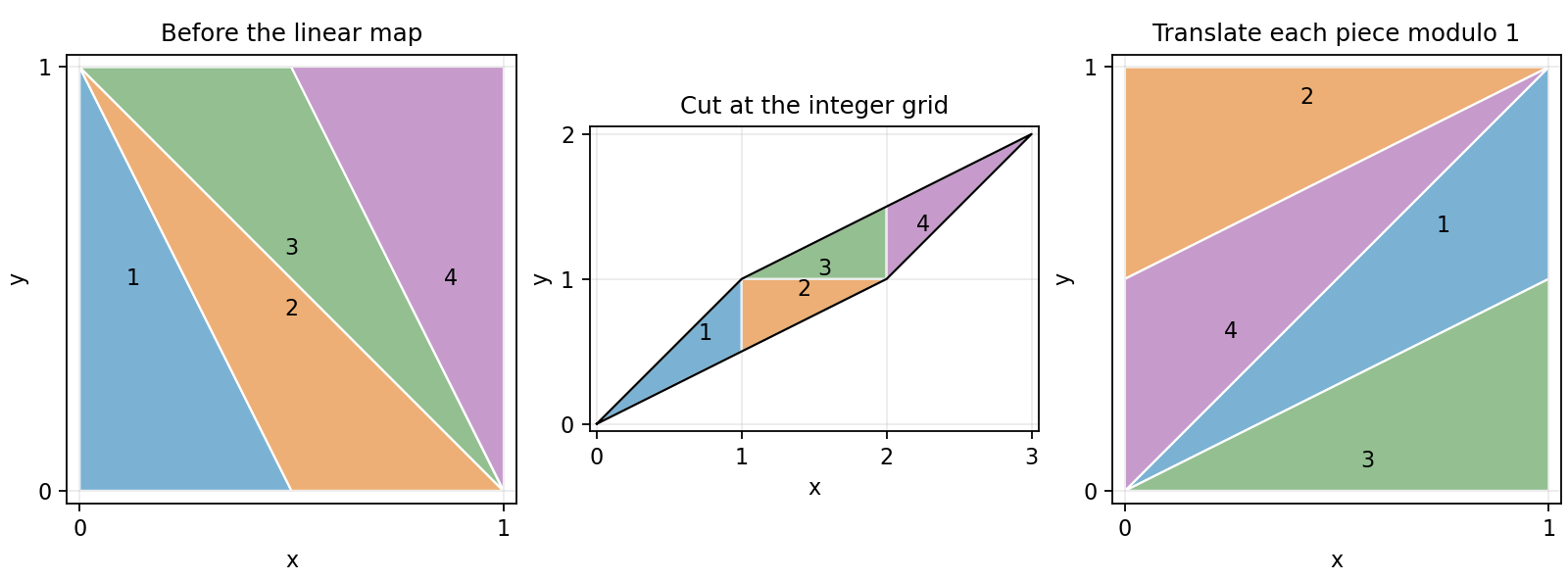
The four vertices of the unit square map to , the vertices of an area-one parallelogram. To reduce it modulo one, cut it by the integer grid. For each piece in the cell , translate by . Up to boundary identifications these translated pieces partition the unit square, because the inverse integer matrix gives exactly one torus preimage to every point. The colored pieces in the original diagram show the same pieces before and after these translations.


For the Fibonacci identity, at the claimed matrix is . If the identity holds at , multiplication on the right by givesEach equality uses , with the specified indexing . This proves the formula for every positive integer .
A fixed point satisfies . Since has an inverse integer matrix, this forces , so the origin is the only fixed point modulo one.
For period dividing two,The second congruence gives ; inserting it into the first gives . Thus the complete list isThe first is the fixed origin. Direct application of exchanges the other four in exactly two pairs:This both verifies the periodic orbits and excludes additional ones.
Finally, if is fixed by , then for an integer vector . The eigenvalues of are and , neither zero. Hence its inverse exists and has rational entries by the adjugate matrix formula for an integer matrix. Therefore has rational coordinates. The derivative of the return map is , with eigenvalues and . Every periodic point is a hyperbolic saddle fixed point of a map and is unstable, although perturbations in its stable eigendirection contract.
For , differentiate and use the two differential equations:Substituting , gives the required equations in polar coordinates. The origin is handled in Cartesian coordinates, where it is an equilibrium point; an angular coordinate is not defined there.
A Lyapunov function near an equilibrium point is a continuously differentiable positive-definite scalar function whose derivative along solutions is nonpositive. This implies local Lyapunov stability under the usual comparison bounds; if its derivative is negative definite, the Second Lyapunov theorem gives local asymptotic stability. Here takeIf , continuity gives a small ball and such that inside it. Consequently . A sufficiently small initial sublevel set stays inside the ball, and . The origin is asymptotically stable, in fact locally exponentially stable. If , continuity instead gives in a small ball. Every nonzero initial point there exits that ball in forward time, proving instability of the origin. These inequalities hold along all local solutions; continuity of alone need not supply uniqueness for a general vector field.
If , a nonzero constant radius satisfying gives a periodic orbit of period , since . Linearizing the scalar radial equation there givesThus the periodic orbit is orbitally asymptotically stable for and unstable for . The direction along the periodic orbit is neutral, as expected for an autonomous periodic orbit; orbital asymptotic stability means attraction in a dynamical system to the orbit with a possible phase shift.
For the specified radial response,The origin is therefore stable for and unstable for . The nonzero-radius equation has roots of an equationretaining only positive radii. For , the square root exceeds one, so only exists and : the periodic orbit is unstable. For , both radii are positive; gives and a stable periodic orbit, while remains unstable.
As increases through , the stable small-radius periodic orbit emerges from the origin while the origin loses Lyapunov stability. This is the supercritical Hopf-type transition with a nonsmooth radial response requested. It follows directly from the explicit radial dynamics. There is a regularity qualification: near zero, so the vector field in Cartesian coordinates contains and terms. It is continuously differentiable but not generally twice differentiable at the origin, and the periodic orbit radius grows as rather than the square-root law of a generic smooth Hopf normal form. One should therefore use the explicit computation here rather than invoke a smooth Hopf bifurcation theorem with unmet hypotheses. At itself the origin is still weakly attracting, because for small positive .
Let . In the first two components of the vector field, replacing by their negatives changes the sign of the whole component; in the third, the product is unchanged. Thus , establishing the symmetry, with solutions mapped to solutions by .
At an equilibrium point, positivity of makes . The remaining equations give and . Hencewhere the two nonzero equilibrium points exist when . They merge with the origin at , in a pitchfork bifurcation.
At the origin the Jacobian matrix and its eigenvalues areAt these are . To see the local pitchfork bifurcation dynamics more explicitly put , , and use on the center manifold. The equations becomeAt , invariance at cubic order gives , hence the reduced equation isIt has the supercritical pitchfork bifurcation form as increases, with the two branches attracting near onset while the origin becomes unstable.
For , the determinant of the planar block is , so the origin has one positive and two negative eigenvalues and is a saddle equilibrium. At , the planar eigenvalues are explicitly . For , the planar trace is negative and its determinant positive, so the origin is asymptotically stable. To distinguish its type putFor both planar eigenvalues are real negative, giving a stable node. At they coincide at ; the planar block is not a scalar matrix, so it is a defective stable node. For they are nonreal with negative real part, giving a stable spiral in the planar block together with the stable third direction. This refines the requested node-versus-saddle classification.
The origin cannot have a Hopf bifurcation: a planar imaginary pair would require trace zero, namely , but the determinant there is , so the pair is real and of opposite signs.
For either nonzero equilibrium point put . The Jacobian matrix isIts characteristic polynomial isA nonzero imaginary root of an equation requires, by separating real and imaginary parts, and . Equivalentlyso the candidate Hopf bifurcation values areAt such an admissible value the factorization is , giving the pair and a negative third eigenvalue , since on the nonzero branches.
The mathematical model parameter restrictions matter. A real candidate requires , and the nonzero equilibrium points also require . The upper-sign value is admissible for ; the lower-sign value additionally requires . For fixed , differentiation of the characteristic equation at the imaginary root of an equation gives the eigenvalue crossing speedThus the transverse eigenvalue crossing condition holds except at the coincident-root case , . At a transverse eigenvalue crossing, a generic nonzero first Lyapunov coefficient gives a Hopf bifurcation. The displayed radical is the spectral threshold; it does not justify an unconditional generic-Hopf claim for all positive mathematical model parameters, nor does it by itself exclude a degenerate Hopf bifurcation point. For example yields no real candidate at all. The cubic Routh-Hurwitz stability criterion gives local Lyapunov stability on the side with and , where
For the modified equation, the planar block at the origin is , with determinant for the stipulated positive mathematical model parameters. Thus the origin is always a saddle equilibrium for nonzero in that mathematical model parameter range. The nonzero equilibrium points now satisfy , and , so they areFor these branches stay a positive distance from the origin and do not merge with it as varies. The origin also has no zero eigenvalue for . Therefore the pitchfork bifurcation is absent in the modified system.
Articles by others on the same topic
There are currently no matching articles.