Past exam of the topics in applied mathematics course of the University of Oxford / 2010 / A / 2 / c

The equal-diffusivity Fisher reduction uses equal diffusion coefficients and the invariant relation $v=1-u$. The second equation then requires $u_{\tau }=\delta u(1-u)+u_{\xi \xi }$, while the first becomes $u_{\tau }=(1-\beta )u(1-u)+u_{\xi \xi }$. They agree whenThis reduction requires compatible initial and boundary data on that invariant relation. Tuning a parameter alone does not force arbitrary solutions of the two-field system onto it. For positive physical $\beta$, the displayed normalization also requires $0<\delta <1$. More generally the line $v=C(1-u)$ works when $\beta C=1-\delta$; the same positivity restriction remains for $C>0$.

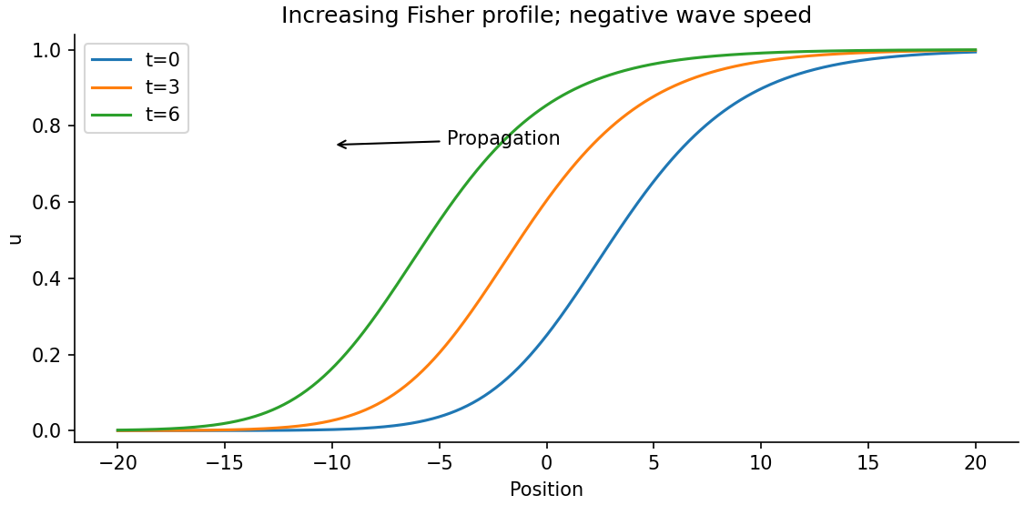
Let $z=\xi -c\tau$ and $u=U(z)$ with $U(-\infty )=0$, $U(+\infty )=1$. The profile equation is $U^{\prime \prime }+c{U}^{\prime }+\delta U(1-U)=0$. Multiplication by $U^{\prime }$ and integration givesConsequently $c<0$: the increasing front moves left, with the $u=1$ state invading $u=0$. Linearization at its leading edge gives real monotone exponents only when $|c|\ge 2\sqrt{\delta }$, yielding the usual Fisher front speed range. A convenient exact example isSubstitution verifies it and the figure shows its leftward displacement. The source uses $x$ for the end limits after defining $\xi$; they denote the same spatial coordinate here.

Yes. An immobile $Y$ concentration can still change locally through reaction while diffusing $X$ transports activation. Vanishing diffusion of one component does not prohibit a propagating reaction front.

In the invariant special case $v=0$, the first equation is already Fisher's equation with growth coefficient one, so it has travelling fronts regardless of $D$. A one-diffuser reaction front also gives a coupled example with nonzero $v$. For $z=\xi -c\tau$, the equations with $D=0$ areFor $0<\delta <2$, choose $k=\sqrt{1-\delta /2}$, $\beta v_0=2-\delta$, and setIndeed $U^{\prime }=kU(1-U)$ and $V^{\prime }/V=-2kU$, giving the second equation. In the first, division by $U(1-U)$ leaves $k^2(1-2U)+ck+1-\beta v_0(1-U)$, whose constant and $U$ coefficients both vanish with these choices. Ahead of the left-moving wave $U=0,V=v_0$; behind it $U=1,V=0$. This explicitly demonstrates a travelling front with substrate depletion but no $Y$ diffusion, rather than relying solely on the uncoupled special case.