This University of Oxford Part B paper covers Mathematical Ecology and Biology in section A and Nonlinear Systems in section B, and is cross-listed for the Mathematics, Mathematics and Computer Science, and Mathematics and Statistics degrees. [ref]
https://www.whatdotheyknow.com/request/maths_past_papers_3. Source release
A bounded search of official sources found no advertised solutions for this exact paper. The complete seven-page archive transcription preserves the printed notation; the solutions explain the initial-data restrictions, omitted Neumann zero modes and zero-frequency exception where needed.For this concave recruitment map, the extinction state is invariant because . Near extinction, with multiplier above one, so small positive populations initially grow. The strict concavity means marginal recruitment decreases as population increases. More precisely, for ,since . Thus per-capita recruitment decreases and the graph bends downwards from an initial slope greater than that of the identity line.
A positive fixed point, if present, is the unique positive intersection with : the strictly decreasing ratio can cross one at most once. The sketch shows the usual saturating example , which crosses at .
The three assumptions alone do not guarantee this crossing. For example satisfies all three and remains strictly above for every . An extra large-population restriction, such as somewhere, supplies existence. Keeping this distinction avoids inventing a carrying capacity that is not implied by the printed hypotheses.
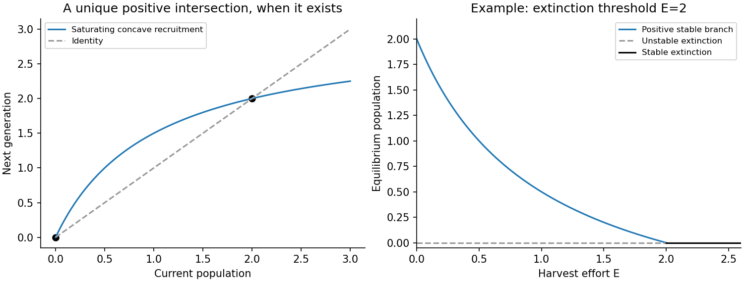
Concave recruitment and the identity line, with loss of the positive equilibrium under harvesting
. Details. Let be a fixed point and put . Taylor expansion gives , so the linear perturbation is . Thereforeis the condition for linear asymptotic stability. A multiplier in gives monotone decay; one in gives alternating decay. If its magnitude exceeds one, perturbations grow. Magnitude one is nonhyperbolic and needs nonlinear analysis.
Strict concavity and already give . Thus the remaining stability requirement is . If is additionally nonnegative on the entire half-line, strict concavity prevents its derivative becoming negative there, since it would then force eventually negative. Under that stronger global population-map assumption the positive fixed point is automatically stable. The printed local slope and concavity information, without that global nonnegativity requirement, does not by itself rule out a flip instability.
With constant-effort harvesting, the constant-effort model isThe extinction multiplier becomes , so extinction is linearly stable when . At its multiplier crosses . Values large enough to make the next population negative lie outside the physical validity of this untruncated harvest model.
Any positive fixed point solves . Since that ratio is strictly decreasing, there is at most one such point, and it decreases with effort. Differentiating the fixed-point equation yieldsIf the unharvested positive branch exists, it continues for and approaches zero as . This follows because its required ratio lies between and ; its intersection lies between zero and the unharvested fixed point. There is no positive fixed point for .
The positive-state multiplier is by concavity. It is stable precisely whenCrossing can change stability through a flip, but the direction of change is not fixed by the three assumptions: has no prescribed sign. In the illustrated saturating example, increasing effort eventually removes the positive branch at extinction. The finite upper stability bound for the algebraic extinction map should not be interpreted as a physically meaningful recovery of a population at unrealistically large harvest effort.
A steady population is a root . To linearize one needs differentiable near that root, an extra local regularity assumption beyond the source's continuity. Setting gives , hence at linear order.
Thus gives linear asymptotic stability and gives instability. If , linearization is inconclusive. In a one-dimensional phase line, the more general nonlinear test is whether the vector field points towards the root from both sides. At the physical boundary , only the right-hand side matters. Continuity alone does not guarantee uniqueness of trajectories, so a standard well-defined flow also presumes a local uniqueness condition, such as local Lipschitz continuity.
The four nonnegative equilibria are . Since all factors are positive below , the sign of on consecutive intervals isThe phase line therefore points away from zero, towards , away from , and towards . Equivalently , and at each simple positive root , . Their signs alternate negative, positive, negative.
Hence extinction and are unstable, while and are asymptotically stable. Initial positive populations below tend to ; those above tend to ; an initial population exactly at remains there. This is bistability with a threshold separating the two basins.
Put . The harvested vector field is . Define the extinction threshold , and let be the positive local maximum of , with . Writing , givesPositive equilibria are intersections of with the horizontal line . A lower stable branch in exists exactly for . A pair in exists exactly for : its smaller member has and is unstable; its larger member has and is stable. At a positive root the linear eigenvalue is , which proves these claims. Extinction has eigenvalue , becoming stable for .
The harvested bistable population thresholds determine the behaviour. If , the upper stable population and its unstable separator first disappear in a saddle-node bifurcation. Populations then tend to the remaining lower stable state until that branch reaches extinction at ; beyond it extinction attracts every positive initial state. If , the lower stable branch reaches extinction first. For , extinction and the upper positive state are both stable, separated by the middle unstable root. Increasing effort through then destroys the remaining positive attractor, causing a sudden collapse to extinction. If , both events occur at the same effort at different populations.
At , near zero the leading term is , so extinction attracts from the physical right side algebraically, despite its zero linear eigenvalue. At , the double positive root is semistable: locally , attracting from above and repelling from below. These critical cases matter for exact initial data. The figure shows examples of both strict threshold orderings.
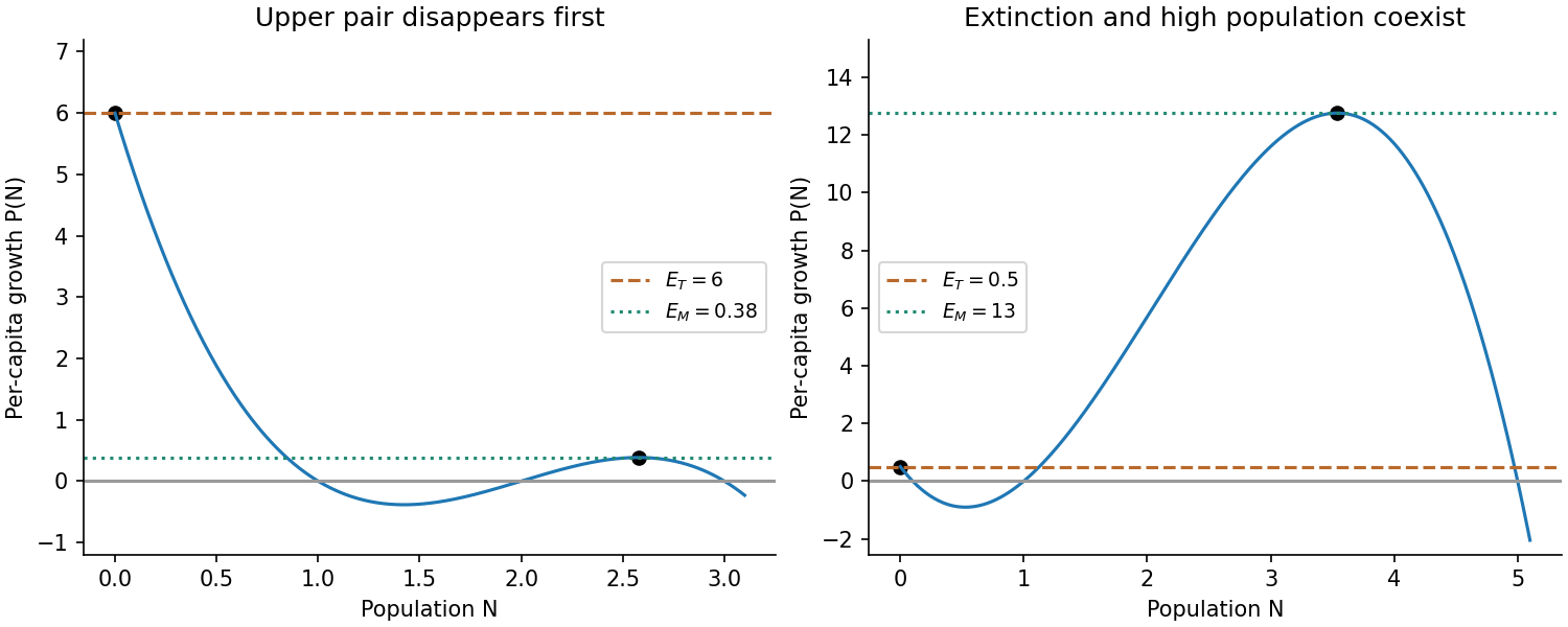
Two possible orderings of the extinction and saddle-node harvesting thresholds
. Details. The law of mass action makes each elementary reaction rate proportional to the product of its reactant concentrations, with the stoichiometric change determining its contribution. Let be maintained constant, and let be the diffusion coefficients. The first reaction consumes two molecules, the second creates one net , the third consumes one each of , and the fourth consumes while creating . Fick's laws for diffusion giveHere the standard deterministic convention takes the event rate of the first reaction as , so its loss is . A convention absorbing a combinatorial factor into leads to the same nondimensional model after consistently redefining that rate constant. The maintained reactant makes this an open chemical model; there is no conservation law requiring to decrease with reaction progress.
Choose , , , and an independently selected positive representing its reference or supplied concentration. Set , , , . Dividing the first equation by and the second by yields the stated system withThe parameter can be changed through the chosen or physically supplied reference concentration while these other combinations remain fixed. The combinations satisfy for this reaction mechanism, so they need not be algebraically independent. The spatial scale makes the diffusion coefficient one, and the time and scales balance linear autocatalytic growth against the quadratic loss.
The equal-diffusivity Fisher reduction uses equal diffusion coefficients and the invariant relation . The second equation then requires , while the first becomes . They agree whenThis reduction requires compatible initial and boundary data on that invariant relation. Tuning a parameter alone does not force arbitrary solutions of the two-field system onto it. For positive physical , the displayed normalization also requires . More generally the line works when ; the same positivity restriction remains for .
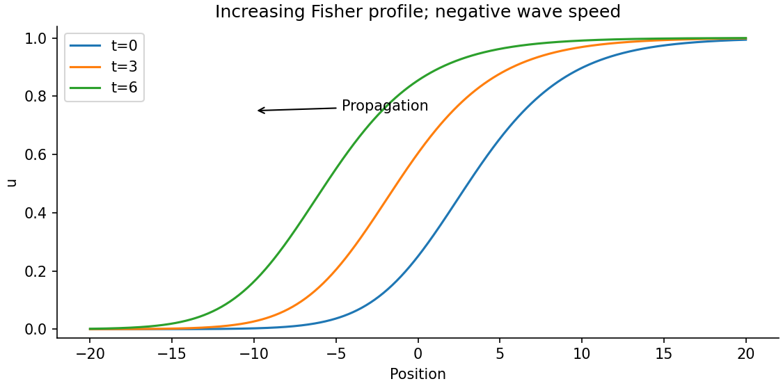
Let and with , . The profile equation is . Multiplication by and integration givesConsequently : the increasing front moves left, with the state invading . Linearization at its leading edge gives real monotone exponents only when , yielding the usual Fisher front speed range. A convenient exact example isSubstitution verifies it and the figure shows its leftward displacement. The source uses for the end limits after defining ; they denote the same spatial coordinate here.


Yes. An immobile concentration can still change locally through reaction while diffusing transports activation. Vanishing diffusion of one component does not prohibit a propagating reaction front.
In the invariant special case , the first equation is already Fisher's equation with growth coefficient one, so it has travelling fronts regardless of . A one-diffuser reaction front also gives a coupled example with nonzero . For , the equations with areFor , choose , , and setIndeed and , giving the second equation. In the first, division by leaves , whose constant and coefficients both vanish with these choices. Ahead of the left-moving wave ; behind it . This explicitly demonstrates a travelling front with substrate depletion but no diffusion, rather than relying solely on the uncoupled special case.
A uniform steady state satisfies . Set , and keep only first-order terms in the perturbations. Since the base state is constant, its Laplacian vanishes. Taylor expansion givesThe zero-flux boundary conditions linearize to homogeneous Neumann conditions, . The off-diagonal entries of the Jacobian describe the cross-effects of the two chemicals, while the diagonal entries describe local self-response.
A diffusion-driven instability means that the homogeneous reaction equilibrium is asymptotically stable against spatially uniform perturbations, but adding diffusion makes at least one admissible spatially nonuniform mode grow. Thus the eigenvalues of must have negative real parts, while has an eigenvalue with positive real part for some positive Neumann Laplacian eigenvalue on the actual domain.
The instability is driven by different diffusion responses acting together with reaction feedback. It is not merely an equilibrium that was already unstable without diffusion. On a bounded domain the permitted wave numbers are discrete, so an algebraically unstable continuous band must also contain an actual spatial eigenmode.
Write , , , , . Stability without diffusion requires and . For a mode with , the characteristic equation isFor positive diffusivities the trace stays negative for every , so growth can occur only if . Put . This upward-opening quadratic has a negative interval at positive exactly when and , orIf , the right side is , impossible. Equivalently diffusion would merely subtract from both reaction eigenvalues. Thus unequal diffusivities are necessary.
The potentially unstable band has endpointsThese are necessary continuous-wave-number conditions. Actual instability on the specified bounded domain additionally requires an allowed strictly between them. The strict inequalities exclude neutral onset and presume both diffusivities are positive, as in an ordinary two-chemical diffusion model.
After relabelling the chemicals if necessary, take and . At least one diagonal entry must be positive because , whereas their sum is negative. Since their product is negative and , the off-diagonal product must be negative and sufficiently large in magnitude. The two possibilities areIn the first, activates its own production and stimulates , while suppresses : an activator-inhibitor mechanism. In the substrate-depletion pattern mechanism, promotes the autocatalytic species , which consumes or suppresses : a substrate-depletion mechanism. These are different biological interaction signs, not merely two drawings of the same feedback. Suitable relative magnitudes and sufficiently different diffusivities are still required; the sign pattern alone does not guarantee a Turing instability.
For Neumann boundaries the correct eigenfunctions include zero indices:Their squared wave number is . The constant pair is reaction-stable. Instability requires , using the band derived above. If both side lengths are large, the wave-number spacings are small enough that admissible modes can enter the band in either direction, including mixed modes. This does not mean the single mode necessarily stays unstable as lengths tend to infinity: its wave number eventually tends to zero below the band. Rather, increasingly fine wave-number spacing permits some suitable higher integers.
Thin-domain Turing mode selection applies if , every mode with has and is stable. A sufficiently large can nevertheless admit an integer with and . HenceThe printed range starting both indices at one excludes these purely longitudinal modes and cannot imply the requested conclusion. It also omits the constant mode. Further, each allowed spatial eigenfunction generally has two temporal eigenvalue branches of , with coefficients along their eigenvectors; a single unrestricted scalar is shorthand for those branches rather than a complete general expansion.
Domain geometry can select biological pattern dimension even when the same reaction parameters and diffusion coefficients are used. A sufficiently wide developing tissue can admit instabilities with variation in two spatial directions; nonlinear development may produce spots, labyrinths or other two-dimensional patterns. A thin strip suppresses transverse unstable modes, allowing primarily bands whose concentration varies along its long axis and is nearly uniform across its width.
This is a mechanism for shape-dependent pattern selection during growth: increasing tissue width can admit additional transverse modes without changing the local chemical interactions. Linear instability predicts initial wavelengths and permitted directions, not the eventual stable spot or stripe pattern; nonlinear saturation and boundary geometry determine that later outcome. Zero-flux boundaries also mean these modes arise through internal redistribution and reaction rather than externally prescribed chemical concentrations.
Let . Every term changes sign when both variables change sign, so . Consequently the derivative of equals , proving the stated rotational symmetry.
This is equivariance under a half-turn, not time reversibility. Reversibility of an autonomous differential equation requires a reverser satisfying , so that is a solution. The half-turn would require , the opposite of what holds. The usual mechanical candidate also fails when damping is present: its second equation would require identically. The symmetry relates two orbits with the same direction of time, and does not reverse their arrows.
The planar divergence is for . Since the plane is simply connected, the Bendixson-Dulac theorem excludes any nonconstant periodic orbit: the flux across a closed trajectory would be zero because the vector field is tangent, whereas Green's theorem makes it the strictly negative integral of the divergence over the enclosed region.
Alternatively define . Direct differentiation givesA nonconstant periodic solution would require the integral of this strictly dissipative expression over a period to vanish. That forces and hence an equilibrium, a contradiction. This energy argument identifies the damping mechanism behind the geometric criterion.
The equilibria satisfy and , giving and . At the origin,Their product is , so the origin is a saddle equilibrium for every real .
At either nonzero equilibrium,The determinant is positive and the trace is . Thus both equilibria are attracting for , repelling for , and have purely imaginary eigenvalues at . More precisely they are stable foci for and stable nodes for ; they are unstable foci for and unstable nodes for . At the two discriminant-zero endpoints they are repeated-eigenvalue degenerate nodes, with a nondiagonalizable Jacobian. At , linearization alone does not determine nonlinear stability or prove a nonlinear centre.
At , the origin has stable and unstable eigenvalues and ; the two nonzero equilibria are repelling foci with eigenvalues . A compatible portrait has one attracting closed orbit surrounding all three equilibria. Its total enclosed index is , as a periodic orbit requires. Its half-turn image is also attracting, so uniqueness of the attracting cycle makes that cycle half-turn symmetric. Orbits spiral away from either focus equilibrium and approach the surrounding cycle; the stable separatrices approach the saddle instead. The figure integrates representative trajectories and shows the local saddle directions.
These trajectories cannot escape to infinity. A Liénard boundedness function supplies one explicit boundedness argument using the Liénard coordinate with and . Then and . Put and . This function is coercive after addition of a constant. Its derivative obeysusing . The right side is negative outside a compact region, yielding bounded forward motion.
In the displayed portrait, generic non-equilibrium initial states tend to the cycle; points on the saddle's stable manifold tend to the origin; and initial data exactly at a repelling focus equilibrium remain there. The Poincaré-Bendixson theorem excludes a chaotic compact limit set for this smooth planar flow. Strictly, the assumption gives uniqueness only of an attracting periodic orbit: it does not by itself exclude exceptional nonattracting periodic or separatrix limit sets. Those would need additional global information if one wanted a classification stronger than the compatible portrait requested.
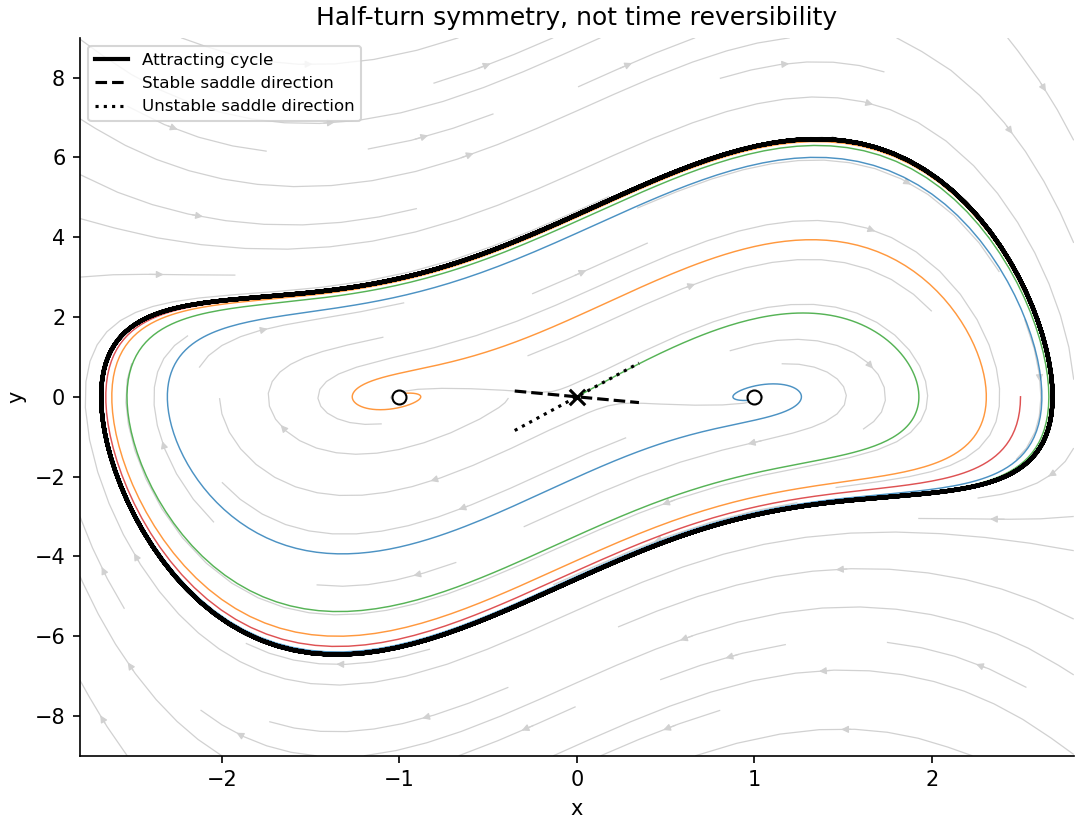
A compatible attracting cycle, repelling foci and saddle separatrices at Omega minus two
. Details. 
First assume and regard modulo . The section has return time . Solving the resonantly forced oscillator from this section givesAt , the sine vanishes and the cosine is one, while differentiating the secular term adds to . Hence the Poincaré map isFor , every iterate has . Thus every oscillator trajectory is unbounded, regardless of its initial amplitude. For an arbitrary section phase , the return map translates by , which is still nonzero. At the map is the identity, and all motions are bounded harmonic oscillations, including the zero-amplitude equilibrium.
The zero-frequency case allowed by the printed parameter range is different. If , then is constant and . There is no phase-crossing Poincaré section. For , choosing and gives bounded equilibria, contradicting an unqualified “all trajectories” statement. For at zero frequency, free-particle motion is unbounded unless . The resonance conclusion therefore requires the natural nonzero-frequency assumption.
For , the fixed points are and when the latter is defined. On the physical interval the nonzero branch exists for , meeting zero at . Their multipliers are and , respectively. Thus zero is linearly attracting for and repelling for ; the positive point is linearly attracting for and repelling for . At and the relevant multiplier has magnitude one, so linearization is inconclusive. At , attracts small positive points to zero nonlinearly.
Factoring and removing its fixed-point factors gives . Its distinct roots areThey map to each other, giving a genuine two-cycle only beyond . The cycle multiplier isSolving in givesAt , the two roots coalesce with , where the fixed-point multiplier is : a supercritical period-doubling bifurcation creates the attracting two-cycle. At the upper endpoint its multiplier reaches , marking the next loss of linear stability. The two-cycle is superstable at , where . At exactly the fixed point remains weakly attracting through higher-order terms: for , the second iterate is , showing alternating perturbations decay slowly.
For a nearby orbit, linearized separation satisfies . Repeated use of the chain rule gives to first order. Taking the logarithm of its magnitude and dividing by gives the exponential growth rateThe infinitesimal-perturbation limit is taken before interpreting long-time growth; finite separations eventually leave the linear regime. The limit is assumed to exist, with a limsup used when needed.
On a -cycle, blocks of successive derivatives repeat. If , the remainder of fewer than terms has vanishing contribution to the long-time average andLinear attraction means , giving . A superstable cycle has , meaning at least one derivative in the cycle vanishes. Its infinitesimal return multiplier is zero and the corresponding logarithmic exponent is . This concerns the derivative cocycle; actual finite perturbations can converge by higher-order rather than literally vanishing in one step.
In the two-symbol shift representation, is fixed under a shift and codes the fixed point labelled . The constant all-ones sequence supplies the analogous example. The dot only marks the present position; shifting it advances one iterate. The assertion uses the faithful orbit coding assumed in the question.
Use the primitive repeating word . One shift changes the sequence and three shifts return it, so the least period is three. A word such as repeated would instead have least period one; primitivity is what distinguishes a true three-cycle from a periodic notation for a fixed point.
The sequence has exactly one and otherwise zero entries. Under forward shifts that exceptional symbol moves out of every fixed observation window; the same happens under backward shifts in the other direction. Thus both temporal limits are the all-zero fixed sequence, while the orbit itself is nonconstant: it is homoclinic to that fixed point. The bi-infinite coding specifies a chosen full orbit even when the original interval map is not invertible.
Choose , with zeros on the entire left tail and ones on the entire right tail. Forward shifts converge in the symbolic metric to the all-one fixed point, while backward shifts converge to the all-zero fixed point. Its two limiting invariant states differ, so it is a heteroclinic orbit. Reversing the two tails reverses these asymptotic roles.
One explicit future itinerary is obtained by concatenating all binary words, ordered first by length and then lexicographically:Extend it arbitrarily to negative indices, for example by zeros. Every finite binary block occurs in its forward itinerary, and indeed occurs arbitrarily far out as a subword of longer words. Its shift orbit is therefore dense in the full two-symbol shift space. It is not eventually periodic: arbitrarily long runs of zeros and ones occur, together with all other finite words.
The full shift has sensitive dependence because sequences agreeing on an arbitrarily large initial window can differ just beyond it, and shifting brings that disagreement into view. Thus this itinerary supplies a dense aperiodic orbit in the chaotic symbolic system assumed by the question. A merely nonrepeating sequence would not be enough: restricted aperiodic sequences can have much simpler, nonchaotic orbit closures. Nor does symbolic description alone assign a numerical Lyapunov exponent without information about the underlying map and its coding.
The Lorenz vector field has constant divergence . Liouville formula for a fundamental matrix for the derivative of the flow therefore givesThis concerns transported three-dimensional phase volume, not the Euclidean distance between each pair of trajectories.
A quasiperiodic orbit with the usual smooth two-frequency torus closure would lie on an invariant embedded two-torus. That torus bounds a solid torus of positive finite volume in . Since the vector field is tangent to its boundary, its outward flux is zero, contradicting the divergence theorem, whose volume integral is . This negative-divergence obstruction to invariant tori excludes such quasiperiodic tori. The argument uses global negative divergence and the enclosed volume; saying only that an attracting torus has zero volume would not exclude it.
At an equilibrium the sum of eigenvalues is , so they cannot all have positive real parts: no equilibrium is a fully repelling source. For a periodic orbit of period , one Floquet multiplier equals one in the flow direction. The product of the other two is , so they cannot both have modulus greater than one: no periodic orbit is fully repelling either. Saddle equilibria and saddle periodic orbits remain possible; contraction of volume does not imply contraction in every direction.
The first equilibrium equation gives , and the third gives . The second then becomes . Hence the equilibria areAt the origin, one eigenvalue is and the remaining two solve . Their discriminant is . For both are negative, so the origin is linearly stable, with all eigenvalues real and negative. For one is positive and one negative, so it is a saddle equilibrium with one unstable and two stable directions. At its eigenvalues are : linearization has a neutral direction and cannot alone prove nonlinear stability. Given the source's global attraction for , there are no nontrivial limit cycles or persistent chaotic invariant dynamics in that regime; all initial states tend to the origin.
To establish the local pitchfork, one needs the simple eigenvalue to cross zero, the two symmetry-related branches to exist and acquire the expected local stability, and nondegeneracy of the nonlinear coefficient. The derivative of the crossing eigenvalue is . At , the characteristic polynomial isFor sufficiently close to one, all coefficients are positive and , so the cubic Routh-Hurwitz criterion makes both new equilibria stable. Together with the symmetry and the square-root branches, this yields the supercritical pitchfork. A local centre-manifold coordinate proportional to has leading normal form , explicitly displaying the nonzero stabilizing cubic coefficient. At that cubic also gives weak local nonlinear attraction along the centre direction.
A useful operational definition of chaos for a deterministic flow is bounded, nonperiodic long-time dynamics on an invariant set with sensitive dependence on initial conditions: arbitrarily close starting states can separate by a fixed macroscopic amount. Boundedness distinguishes recurrent irregular dynamics from simple exponential escape; aperiodicity excludes a limit cycle; sensitivity distinguishes chaotic unpredictability from a regular quasiperiodic signal. These are properties of the asymptotic dynamics, not a short irregular transient. One precise topological convention, Devaney chaos on a compact invariant set, instead specifies topological transitivity, dense periodic orbits, and sensitive dependence. Transitivity expresses indecomposability of the recurrent motion, while dense periodic orbits mean every region contains unstable recurrent structure. The convention should be stated because these formulations are not identical in complete generality.
An attractor is an invariant set approached by trajectories from a neighbourhood or positive-measure basin, according to the adopted attractor convention. Calling it strange refers to irregular, typically fractal geometry rather than a smooth point, cycle or torus. Strangeness alone does not force chaos. Strange nonchaotic attractors provide counterexamples: geometrically irregular attracting sets can lack positive exponential separation. Primary examples appear in [ref]
https://doi.org/10.1016/0167-2789(84)90282-3. Strange attractors that are not chaotic, Physica D 13 (1984), pages 261–268
. This geometric convention does not assert that every such example occurs in the autonomous three-variable Lorenz family.Two complementary numerical diagnostics are to estimate the largest Lyapunov exponent and to construct a return map. For the first, integrate the variational equation alongside the Lorenz trajectory, repeatedly normalize , and average the logarithms of the accumulated stretch factors after discarding a transient. A positive converged exponent suggests sensitive exponential separation; the full spectrum should include a zero flow exponent and have sum , providing checks. For the second, record transverse crossings of a Poincaré section or successive maxima of a state variable, then look for the stretching and folding of an aperiodic return set rather than one point or a finite cycle. Nearby-orbit separation or a broadband power spectrum can add evidence, but plots alone do not prove chaos. Repeat with smaller integration step, longer runs and several initial conditions to distinguish numerical error, long transients and coexistence of attractors from persistent dynamics.
Articles by others on the same topic
There are currently no matching articles.