Section E: Mathematical Tools.
There are four well-mixed reservoirs: Mediterranean surface/deep and Black Sea surface/deep . Use the actual drawing’s arrow endpoints: leaves , enters from , and starts in and enters . With as positive water-mass transport rates, the four steady conservation of mass equations areAdding them cancels every internal transport and gives the whole-system requirement . There is no stated evaporation, precipitation or other external transport to add.
The schematic endpoints are unusual for the conventional two-layer exchange picture: its Gibraltar outflow is drawn in the surface box, and its Black Sea surface inflow descends into the Mediterranean deep box. Moving to , to , and the source of to would define a different, more conventional idealization. The displayed equations consistently follow the supplied drawing; the same endpoint convention is used in the following two parts.
Let be salt mass fractions, with reservoir water masses denoted by the corresponding symbols. Let be Atlantic inflow salinity and the Danube inflow salinity, approximately zero for fresh water. With the diagram endpoint convention from part i, instantaneous mixing givesEvery outgoing salt transport uses the salinity of its donor box. The water masses are constant because the water balances are at steady state, even while the salinities evolve. If reservoir water masses varied, the left side would instead be .
Summing yields , a direct whole-system salt check. Fresh water carries essentially no salt, but its dilution effect is still present through the water balance and the resulting transport terms.
For a constant-mass, well-mixed box the mean residence time is stored water mass divided by its total outgoing water-mass transport. Using the source figure’s endpoints,At water steady state, each denominator can equivalently be replaced by that box’s summed inflow. If transports are specified as volume rates, use volume rather than mass in the numerator, or convert with density consistently. The drawn maximum basin depths alone do not supply layer volumes, plan areas or transport magnitudes, so no numerical residence times follow. Internal recycling counts as exit from a particular box; these times are not the time to escape the combined sea system.
Write . For , direct partial differentiation givesHence exactly when , proving the claimed diffusion equation solution. At , , so . The infinite spatial domain needs no end-boundary conditions. For positive thermal diffusivity the amplitude decreases, as described by the thermal diffusion rate of a Fourier mode.
Choose to make the sketch explicit. The three profiles areThey have the same wavelength, zero crossings and phase, with amplitudes , and . Diffusion reduces the temperature gradient and amplitude; it does not advect or change this individual mode’s wavelength.
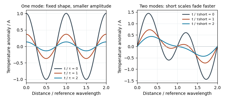
Original diffusion solutions: one Fourier mode loses amplitude, and a two-mode profile loses its short-wavelength structure faster
. Details. 
The diffusion equation is linear, so superposition givesEach term separately satisfies the equation, and their sum recovers the stated initial data at . Its e-folding times are , so implies . The shorter-wavelength oscillation loses a given fraction of its amplitude first. It approaches zero exponentially rather than disappearing at a finite instant. This preferential damping explains smoothing of fine-scale temperature structure.
For an integrable initial profile , use its Fourier transform with the conventionThe transformed diffusion equation is , soEquivalently the heat-kernel convolution isThis also accommodates bounded piecewise-continuous initial profiles; it recovers at continuity points as . For periodic initial data use a Fourier series and multiply each mode by ; the constant mean mode remains unchanged. “Any function” needs the usual existence/integrability or growth conditions: an arbitrarily fast-growing initial function need not give a finite heat-kernel integral.
Sampling at Hz means s. The target times are therefore , and s, all within the supplied observation range. For bracketing observations, linear interpolation gives . ThusThe estimated displacements are , and . Interpolation assumes approximately linear behavior within each interval; it does not recover any unobserved high-frequency motion.
Regular timing supplies a common interval and a well-defined frequency grid for a standard discrete Fourier transform and Fast Fourier transform. It also makes sample-index lags correspond to fixed physical delays in cross-correlation, autocorrelation and digital filtering. These methods estimate frequency content and characteristic periods, separate instrument or environmental noise from signals, identify arrivals and time delays, and compare ground-motion spectra.
A uniform interval establishes a Nyquist frequency; frequencies above it alias unless filtered before acquisition. Interpolating irregular data onto a regular grid does not undo prior aliasing or fill large gaps with new measurements, and it can alter spectra and create correlated errors. Methods that directly use irregular times are possible, but the ordinary FFT and fixed-lag filter formulas cannot simply treat the original irregular observations as evenly spaced.
Successive jumps occur at times separated by s. Between and s the plotted function is , periodically extended, with maximum and minimum . Its mean is therefore m, and is an odd function over that centered period.
For the Fourier series convention m and for every ; the nonconstant content consists of sine terms. If denotes the mean directly in the alternative convention , its value is m. Stating the convention resolves the otherwise ambiguous notation.
Articles by others on the same topic
There are currently no matching articles.