Source release: Oxford Earth sciences examination release. The held paper is dated 2 June 2022. Both supplied attachments are used below, and all twelve questions across the six sections are solved.
A normal fault is the plausible interpretation. The photograph shows a steep, exposed planar rock face with lower ground on its open side; this geometry is consistent with an exhumed footwall and a down-dropped hanging wall. A steep dip alone is not a unique indicator of shear sense, and the photograph does not supply a displaced marker proving the sense independently. Under an Andersonian faulting regime, a plausible maximum compression is approximately vertical, with horizontal in the extension direction and approximately along strike.
A numerical answer needs an assumption about fault orientation. For a cohesionless fault optimally oriented for Mohr-Coulomb failure criterion, with vertical , write for the internal friction angle and for the fault dip. The angle between the plane and is , so the optimal normal-fault dip relation givesHence under that model.
For the Mohr circle, plot effective compression horizontally and shear stress vertically. Draw a circle with diameter tangent to . Its centre and radius obey . One illustrative normalization is , , with tangency at the resolved stresses on the plane. Pore fluid pressure shifts the total-stress circle horizontally; the friction law uses effective stress.
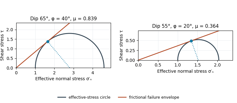
Original normalized Mohr circles for optimally oriented normal faults: different dips imply different tangent slopes only under the stated failure model
. Details. 
The dip does not determine the actual sliding coefficient of friction without the optimal-orientation assumption. A reactivated inherited plane may be nonoptimal, cohesion may matter, and the stress ratio and pore fluid pressure are not measured. For an arbitrary compression-positive stress state,at cohesionless sliding. Thus the requested single value is a conditional inference, not a friction measurement.
The visible surface can be an exhumed fault surface, rather than an unrelated hillslope that happens to intersect a buried plane. Downward motion of the hanging wall exposes the footwall face; repeated displacement and removal of loose material can reveal a substantial length of the same fault plane. Where exposure is renewed faster than weathering, erosion and collapse erase it, that planar surface remains part of the hillside. The less weathered lower face and rougher, vegetated upper ground are consistent with differential exposure, though the photograph alone does not date individual events.
At greater distance or over longer times, erosion modifies the slope and the hillside will cross or obscure the fault plane. The correspondence is therefore a transient competition between fault slip, exhumation and surface processes, not a requirement that all hillslopes follow faults.
Assuming pure dip-slip faulting, use an east–west striking, north-dipping normal fault, with the northern hanging wall moving down dip. In a right-hand-rule strike convention this is strike , dip , rake . The auxiliary nodal plane strikes east–west and dips south. The focal mechanism has a predominantly vertical P axis and a predominantly north–south horizontal T axis; the steep central direction is dilatational.
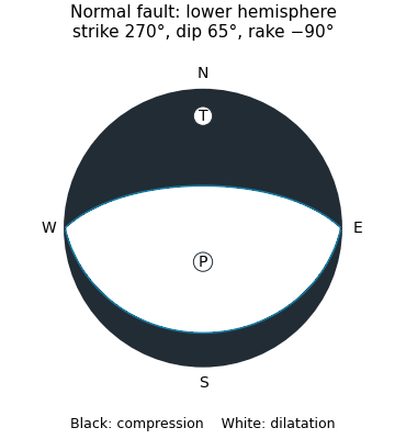
Original lower-hemisphere normal-fault focal mechanism: black compression, white dilatation, and two alternative nodal planes
. Details. 
The sketch is a double-couple seismic moment tensor calculation, not a claim that first motions uniquely identify which nodal plane slipped. The mapped north-dipping surface supplies that additional geological choice.
The along-strike rupture time is , where is rupture velocity. Taking a representative crustal gives about s for a km unilateral finite-source rupture. A different assumed rupture velocity changes this estimate. The local slip rise time at one patch is not specified and need not equal the whole-fault rupture time.
For comparable distance and ground conditions, the eastern observer lies in the forward rupture directivity direction. Radiation from successive patches arrives closer together, producing a shorter, more concentrated and generally larger-amplitude ground-velocity pulse. The western observer receives the contributions spread over a longer interval, generally with less concentrated shaking. This concerns pulse duration and amplitude; it does not imply an equally large permanent displacement at the eastern site.[ref]
What is Directivity by United States Geological Survey. Explanation of constructive interference and the relation of rupture speed to S-wave speed
For distant observers approximately along strike, an elementary seismic travel time construction giveswhere is the shear-wave velocity. With and , these propagation contributions are about and s, respectively; finite local rise time broadens them. Double-couple radiation pattern, receiver geometry and local site response can change the observed amplitudes, so location east or west alone is not an unconditional intensity prediction.
For an Andersonian faulting regime appropriate to the stated normal fault, take vertical, north–south along strike, and east–west. Thus the minimum horizontal compression is normal to the fault’s north–south strike. In an east–up cross-section, draw vertically and horizontally, with perpendicular to the page. These are plausible regional principal stress directions, rather than measured directions uniquely recoverable from one photograph.
Use the same conditional optimal normal-fault dip relation as in question 1, with :The second panel of the original Mohr circle figure has and ; its tangent from the origin has slope . Resolving the stresses onto a plane places its stress point at that tangency. The diagram assumes negligible cohesion, a vertical maximum principal stress and an optimally oriented new or equivalently oriented sliding plane. Without those assumptions, a dip and a statement that sliding began do not uniquely determine the coefficient of friction.
Choose coordinates and use compression-positive effective stress. One possible tensor, in MPa, isIts ordered principal stresses are vertical , north–south and east–west . On the east-dipping plane,so , as required by the conditional friction estimate. The scale is illustrative: no absolute stress magnitude is supplied. A corresponding total stress tensor is for any specified isotropic pore fluid pressure .
The thin, pale, steep feature beside the fingers is plausibly a mineral-filled opening fracture, a mineral vein, rather than the whole coarse fault breccia band. Calcite is a plausible filling in this appearance, but its mineral identity would need a field or laboratory test. Opening normal to its approximately vertical north–south plane requires the smallest principal stress to be approximately east–west, consistent with the extension direction above.
For example, a compression-positive effective stress tensorhas east–west tension and can open a weak fracture whose tensile strength is at most MPa. More generally opening requires , where is tensile strength. This illustrates hydraulic opening of a mineral vein: raising by MPa at the illustrative total stresses in part c translates all effective principal stresses by MPa, producing this tensor without rotating its axes.
The vein and fault slip need not have formed simultaneously at those exact magnitudes: pressure transients, local stress changes and slip can alternate. Their orientations can nevertheless reflect the same normal-faulting stress regime. The source’s reference to “part d” is circular; the meaningful comparison is with part c.
The coarse angular fragments in the light-coloured band identify a fault breccia, probably cemented and accompanied by finer comminuted material. Repeated brittle fracture, clast rotation and crushing during fault slip produce the fragments; fluid flow can later fill pores and fractures with mineral cement. If the finer material is cohesive it can be termed cataclasite; a loose, very fine seam is fault gouge. The photograph alone does not establish all those cohesion and grain-size distinctions.
Slip is commonly concentrated on a narrow principal slip surface or fine-grained seam at a margin or inside a broader damaged band. Thus the coarsest, widest breccia is not automatically the material that accommodated the largest shear displacement. In this image the sharp, finer-looking boundaries of the coarse band are the best candidates for localized slip. Identifying the uniquely most displaced seam would require displaced markers, thin sections or additional exposure; the coarse band itself records substantial distributed damage.
Section B: Remote Sensing & Active Tectonics.
For regional coverage, use stereo photogrammetry from overlapping satellite or airborne imagery, or a radar-derived digital elevation model where suitable data exist. Match the same terrain features in images taken from different known viewing positions, infer their three-dimensional positions by triangulation, and georeference and grid the result. Satellite stereo or interferometric radar can cover efficiently; choose pixel size and vertical precision fine enough for the fault scarps of interest, rather than assuming every regional model resolves small scarps.
InSAR topographic mapping uses the phase difference from a known viewing baseline; repeat-pass deformation work must separate that height contribution from actual motion. Vegetation, cloud, radar shadow and steep slopes can leave gaps or represent the canopy rather than bare ground.[ref]
Interferometry by NASA. Topographic mapping with separated viewing positions and the known baseline; DEM construction
Ground control and independent elevation checks are needed before interpreting small relief as active faulting.Use airborne lidar with sufficient pulse density and ground-return classification. Laser travel times give ranges; the aircraft’s surveyed position and orientation place returns in three dimensions. Multiple returns include canopy and, where gaps permit, the ground. Classify ground points, remove vegetation returns and interpolate a bare-ground digital elevation model over the strip.
This specifically addresses the forest-obscured fault scarp, unlike ordinary optical stereo, which primarily models the visible canopy. Leaf-off acquisition can improve ground sampling where relevant. Dense understorey and a complete lack of ground returns still cause uncertainty; interpolation does not create observed ground heights. Inspect ground-point coverage and compare hillshades under several illumination directions.[ref]
What is the difference between lidar data and a digital elevation model by United States Geological Survey. Point clouds, vegetation removal and the bare-earth product
Use low-altitude structure-from-motion photogrammetry, with strongly overlapping aerial images and well-distributed surveyed ground control points. Bundle adjustment estimates camera geometry and a dense surface reconstruction; independent check points test its accuracy. A small unmanned aircraft or carefully controlled close-range aerial platform can cover the site with centimetre ground sampling. Surveyed targets and stable camera calibration are essential: centimetre pixels alone do not establish centimetre vertical accuracy.
For exposed trench walls or especially demanding local geometry, terrestrial lidar is an alternative or complement. Remove vegetation where permissible, retain the trench’s sharp topographic breaks and state whether the output is a visible surface model or a bare-ground digital elevation model.
Use normalized image coordinates within the map rectangle, with at its upper left and at its lower right. A principal candidate thrust fault trace follows the sharp, approximately diagonal southwestern edge of the dissected high ground on the right: a practical tracing guide passes nearMark the upland, upper-right side as hanging wall and the smoother, lower-left basin side as footwall for a thrust dipping beneath the uplands. Use broken lines through the gaps, not one asserted continuous exposed rupture. A subsidiary candidate frontal segment follows the basin-facing edge of the isolated dissected ridge on the left, approximately through to ; place teeth toward its locally higher ridge side.
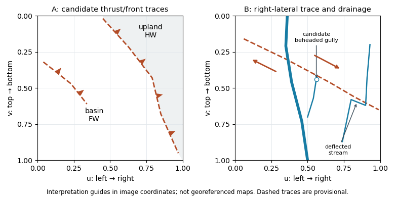
Original interpretation guides for both attachments: provisional traces, block motion and drainage markers in normalized image coordinates
. Details. 
These are geomorphic interpretations of mountain fronts and scarps, not measured subsurface dip directions. On a conventional north-up reading the principal trend is broadly northwest–southeast, but the supplied map has no north arrow: the image-relative coordinates are the reproducible identification. Southwestern illumination means southwest-facing slopes are bright; brightness is a slope-orientation clue, not an elevation contour. Some aligned relief may be a fold scarp or an eroded lithological contact, so field confirmation and topographic profiles would test the candidate traces.
After removing orbital, topographic and atmospheric contributions, an earthquake InSAR radar interferogram would show elongated displacement lobes and generally closed or nested fringes associated with uplift and horizontal shortening of the hanging wall. Each full phase cycle represents of line-of-sight displacement, where is radar wavelength; equivalently , with sign fixed by processing convention.[ref]
Interferometry by NASA. Phase differencing, nuisance contributions and half-wavelength displacement per fringe
If primary slip reaches the surface, expect a displacement discontinuity across the surface trace: fringes can terminate or change abruptly there, and large near-fault gradients or disturbed ground may decorrelate. For a blind reverse fault, the elastic displacement field is continuous at the ground surface and spread over a broader zone, giving smoother gradients and fringes over the uplifted fold. A blind rupture can still create sharp local gradients or secondary faulting.
The exact colour order, number of fringes and sign of the displacement lobes cannot be fixed from this shaded relief alone. They depend on slip, depth and radar look direction; uplift is only one contribution to line-of-sight displacement.
A blind reverse fault can shorten and bend its cover into a fault-propagation fold or other growing anticline. At the fold crest, bending can create shallow extension and secondary normal faults or tension fissures, even though the regional deformation is shortening. Bedding-parallel flexural slip, local backthrusts and fold scarps can also break the surface.
Thus a shallow surface break need not be the upward continuation of the main seismogenic thrust fault. The expected association is distributed deformation related to the uplifted fold; its detailed pattern depends on cover layering, fold geometry and shallow strength. The broad frontal relief in Attachment A is compatible with this possibility, but the image alone does not establish a unique earthquake rupture history.
Section B: Remote Sensing & Active Tectonics.
Many optical land-mapping missions acquire daylight images in the midmorning, roughly 10–11 local solar time, using a Sun-synchronous orbit. This supplies substantial solar illumination while often avoiding the stronger afternoon convective cloud development. It also gives useful relief shadows without the very long shadows and weak illumination of sunrise. Repeated local-time viewing reduces illumination changes when comparing scenes.[ref]
Catalog of Earth satellite orbits by NASA Earth Observatory. Low Earth Orbit: repeated local solar time and the approximately 10:30 morning example
The time is a mission design choice, not a law applying to every optical satellite; afternoon acquisitions also exist. Sun-synchrony approximately fixes local solar time, not the same civil clock time everywhere, and seasonal solar-angle changes remain.
A band ratio image emphasizes differences in spectral reflectance rather than overall brightness. If two corrected band signals are and , with the same multiplicative illumination factor , their ratio is : common shading or exposure factors cancel. Materials with different spectral slopes or absorption features can therefore separate more clearly than in either band alone.
The cancellation is approximate. Additive atmospheric path radiance, different angular reflectance responses and different band noise do not cancel, and division by a small denominator amplifies errors. Use calibrated, co-registered bands and mask cloud, deep shadow and invalid pixels before interpreting a ratio as a material or vegetation contrast.
Use a near-infrared/red ratio, or its normalized form, the normalized difference vegetation index:Useful bands are approximately – in red and – in near infrared, with exact ranges depending on the sensor. Chlorophyll absorbs strongly in red, whereas leaf structure scatters near infrared efficiently; healthy green vegetation therefore has a large near-infrared/red ratio and positive NDVI. Soil and water have different spectral contrasts.[ref]
Measuring vegetation by NASA Earth Observatory. Normalized Difference Vegetation Index: visible absorption, near-infrared scattering and the normalized ratio
A single value is not a direct census of vegetation biomass or species. Soil background, canopy saturation, season, atmospheric effects and mixed pixels need consideration when mapping the distribution of vegetation.
Trace the subtle, approximately straight strike-slip fault that cuts across the dissected fan surfaces, descending to the right in the image. In normalized map coordinates measured from the upper left, a tracing corridor runs approximately from through , and toward . The broad central river interrupts the surface expression; extend the trace across that gap cautiously rather than following the river downstream.
The systematic jogs of small channels, particularly the conspicuous right-hand drainage, support right-lateral strike-slip faulting: draw arrows parallel to the trace, with the upper-side block toward the image right/down and the lower-side block toward the image left/up. Restore paired channel segments by reversing that sense and check that the fan rills align better. An isolated channel bend can have an erosional origin, so the consistent set of bends is stronger evidence than any one bend. No cardinal azimuth is asserted because Attachment B provides no north arrow.
A useful deflected stream is the conspicuous incised drainage in the right-hand part of the image. It approaches the fault corridor from the upper-right, follows a short segment along the trace near , then resumes down the fan toward the lower-left. Mark the two bends and the intervening along-fault reach, rather than labeling the whole channel as a fault.
A candidate beheaded stream is the short downstream gully in the fan immediately to the right of the central wide river, near : its head terminates at or near the cross-cutting fault corridor without an obvious continuation into a substantial upstream catchment. Mark it as a candidate abandoned/cut-off channel, and distinguish it from the active continuous drainage farther right. A displaced upstream counterpart, sediment infill or a field profile would strengthen that identification; optical appearance alone cannot uniquely establish every former channel connection.
If a restored channel or fan boundary has accumulated displacement since it formed, a constant fault slip rate gives the geomorphic offset-age relationThe right-hand channel jog is of order one to two of the printed m scale bars, so apparent offsets of order – m give about – ka. These are scale-based order-of-magnitude estimates, not surveyed piercing-point offsets: the amount of deflection along an eroding channel is not automatically equal to the tectonic displacement. For example, a reliably restored m marker would imply ka.
These times lie in the late Pleistocene, when global glacial–interglacial changes could alter vegetation, sediment supply and runoff and thereby promote alluvial fan deposition or abandonment. The wide interval spans different climatic phases, so it does not identify one event or prove a climatic cause. More importantly, a channel cut into a fan usually dates channel establishment or abandonment; the fan sediment can be older. Independent optically stimulated luminescence dating, stratigraphic correlation and several matched offsets are needed to assign a depositional age and test a climatic correlation.
Section C: Geophysical Methods.
A gravity anomaly is measured gravity minus a specified reference gravity after the stated reductions. A Bouguer gravity anomaly aims to remove the predictable effects of latitude, observation elevation and surrounding topographic mass, so residual variations can be related to subsurface geophysical density contrasts.
Measure relative gravity with a calibrated gravimeter at stations across and beyond the crater, and survey station positions and elevations accurately, preferably with GNSS tied to a reference datum. Repeat a base station through the day to estimate instrument drift and tie the traverse to a gravity datum. Record station times, because tidal and drift corrections are time dependent.
Apply instrument scale and drift corrections, solid-Earth and relevant ocean-loading tidal corrections, latitude/reference-ellipsoid gravity subtraction, the free-air correction, the Bouguer slab correction for material between station and datum, and a terrain correction for departures from a flat slab. The crater’s strong relief makes the last correction important. A local regional-field/background estimate is also needed if the target is the crater’s residual anomaly. State the reduction density; it is not the inferred breccia density.[ref]
Geophysical Data Grids for the Conterminous United States by United States Geological Survey. Gravity-anomaly discussion: latitude, free-air, simple Bouguer and terrain reductions
For a fixed land traverse there is no moving-platform Eötvös correction to add.Treat the quoted anomaly as the response of a slab of thickness replacing host rock. The Bouguer slab formula applies to the geophysical density contrast, not the absolute density:With , m and ,Thus in the slab approximation. The negative anomaly requires less dense infill. A finite bowl has a different geometric response, and water, post-impact sediment and the regional baseline can matter; the stated calculation is the requested slab estimate. The plotted minimum appears closer to mGal, but the numerical instruction explicitly supplies mGal and controls this calculation.
Collect a magnetic survey along the traverse with a calibrated total-field magnetometer, recording time, accurately surveyed position and sensor height. Extend observations beyond the crater to establish the background, repeat stations or tie lines to test consistency, and use a stationary base-station magnetometer to monitor temporal field changes. Keep the instrument away from vehicles, fences and magnetic equipment; map unavoidable cultural sources rather than treating them as geological signals.
Correct instrument offsets and heading effects where applicable, remove measured diurnal variation, reject or separately treat magnetic-storm intervals, and subtract the appropriate large-scale geomagnetic field at the survey epoch. Level overlapping traverses and state whether a local regional trend has also been removed. Unlike gravity, there is no universal rock-independent Bouguer correction for magnetic topography: a magnetic topographic effect needs a model of terrain and magnetization.
Measure representative magnetic susceptibility and remanent magnetization on oriented rock samples to interpret the profile. Total field alone does not tell whether a contrast comes from induced or remanent magnetization, crater excavation, or strongly magnetic material in the infill.
At low northern latitude, a simple induced total-field magnetic anomaly is generally asymmetric and bipolar, not a symmetric central positive peak. A compact body more magnetic than its surroundings, magnetized parallel to a northward, downward ambient field, gives its principal positive lobe on the southern side and a negative lobe toward the north. At exactly zero magnetic inclination its central anomaly reverses relative to the pole; latitude and survey orientation must therefore be included.[ref]
Magnetic line profiles by UBC Geophysical Inversion Facility. Line-profile examples 1–5: latitude, profile orientation and remanence effects
For an original explicit sketch, put a dipole at depth and let increase northward. In a north–south vertical section with inducing inclination , an induced magnetization parallel to the ambient field givesA geocentric-dipole approximation at latitude gives , only an illustrative field direction, not a measured local value.
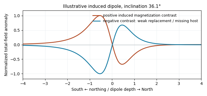
Original induced-dipole profiles: a positive magnetic body and an excavated or weakly magnetized replacement give opposite signs at the same field inclination
. Details. 
For the actual crater, breccia, water and sediment may replace more magnetic basalt, giving negative magnetization contrast. In that case reverse the simple positive-body sketch: a dominant southern low and a northern high are possible even with purely induced contrasts. The magnetic sign cannot be inferred from density or from the word “crater” alone.
The supplied south–north profile has a large southern/interior negative trough and a sharp positive peak toward the northern rim. That is opposite to the simplest positive, presently induced magnetic body in question 5(d). It therefore does not justify interpreting the crater as a concentration of strongly magnetic meteorite material.
A negative magnetization contrast from replacing magnetic basalt already reverses the simple induced-body response. In addition, the target Deccan Traps can retain strong remanent magnetization whose direction differs from the present geomagnetic field; crater excavation and rim geometry then produce a strong magnetic topographic effect. Rock-magnetic measurements and forward modelling distinguish these contributions. A primary study of this crater attributes most of its anomaly to magnetized target basalts and topography, with a comparatively small contribution from the breccia and post-impact sediment.[ref]
The curve alone is not a unique diagnosis of reversed polarity, impact-induced magnetization or a buried iron mass. The physical conclusion supported by the comparison is that a positive induced-body model is inadequate; inherited target-rock magnetization, its removal and geometry must be modelled.
Section C: Geophysical Methods.
For an approximately isotropic elastic solid,where is bulk modulus, is shear modulus and is mass density. Five relevant controls are:
- Mineral composition and texture: different elastic moduli and densities give different seismic velocities; compliant clay-rich material generally differs from crystalline igneous framework rock.
- Porosity, cracks and fractures: compliant voids reduce the effective moduli and usually reduce both speeds; aligned fractures produce seismic anisotropy.
- Effective confinement: increasing effective stress closes compliant cracks and tends to raise speeds. Higher pore fluid pressure at fixed total confinement can reopen or preserve cracks and lower the effective stiffness.
- Fluid saturation and phase: replacing gas by liquid commonly increases the saturated bulk modulus and ; fluids have no static shear rigidity, so changes through the frame, density and frequency-dependent interactions rather than a direct fluid shear modulus.
- Temperature and alteration: heating commonly reduces elastic moduli and may create thermal cracks; hydrothermal alteration can replace strong minerals by clay or other weaker phases. The sign depends on alteration products and crack sealing, so reservoir-specific measurements are needed.
These controls interact: a dense rock is not automatically faster if its moduli are also different.
The reflected P wave remains in the upper layer. Conservation of horizontal seismic ray parameter gives , so the reflected P angle is from vertical. This is specular reflection at the horizontal interface.
For the converted reflected S wave, Snell law for elastic waves givesThus from vertical, in the upper layer. The converted in-plane mode is SV; an isotropic planar P incidence does not generate an independent SH mode.
The required transmitted P wave angle would satisfyTherefore there is no real transmitted P-ray angle. The incidence exceeds the P critical angle ; the transmitted P contribution is evanescent away from the interface rather than a propagating body ray. Reporting would describe critical incidence, not the stated incidence.
The transmitted converted S wave obeysHence from vertical. A propagating transmitted SV mode can exist even though the transmitted P mode is already supercritical.
At P critical incidence the transmitted P wave travels along the interface. The common horizontal seismic ray parameter is , givingThe resulting seismic head wave radiates back into the slower upper layer.
For a converted lower-layer S wave head wave, set the transmitted S angle to :This is possible because . It is the incident P angle needed for the converted SV branch to become tangential, not an S incident angle in layer 1.
The normal-incidence acoustic impedance is . ThereforeThese are and MRayl. They combine the material’s density and wave speed; using would give shear rather than acoustic P impedance.
Specify the amplitude convention. For normal-stress/pressure amplitudes, the seismic reflection coefficient and seismic transmission coefficient areFor particle displacement or velocity resolved in one fixed normal coordinate, the reflected amplitude changes sign and the transmitted ratio is insteadThese are alternative conventions, not conflicting energy predictions. The reflected and transmitted energy flux fractions arewhich sum to one for the ideal lossless interface. Thus an amplitude transmission coefficient greater than one does not violate conservation of energy.
An explosive seismic source gives an impulsive, potentially high-energy broad-band signal and can couple effectively to competent material. It can be useful where strong penetration is needed and heavy vibrating vehicles cannot reach the site. Disadvantages include destructive ground disturbance, permitting and specialist handling, variable source coupling and signature, and the cost of repeated source preparation. The comparison does not require a prescription for charge size or emplacement.
Vibroseis spreads controlled energy over a longer frequency sweep. It is repeatable, permits tailored bandwidth and repeated sweeps, and its known signal supports correlation processing and rejection of unrelated noise. It avoids the impulsive ground disruption of an explosive source. Disadvantages include vehicle access and terrain restrictions, dependence on baseplate coupling, limited force and low-frequency performance, possible harmonic distortion, and strong near-surface waves. For a fractured shallow geothermal site, test which source produces usable coherent reflections or arrivals in the desired band; nominal source energy alone does not establish data quality.
At each source position, couple the vibrator to the ground, transmit a known frequency sweep and record the ground response on synchronized geophones. Record a pilot or measured source-force reference and sufficient listening time for delayed arrivals. Repeat sweeps where beneficial and retain geometry and timing information.
If the Earth’s impulse response is , a linear model is . Vibroseis correlation cross-correlates the record with the known sweep:The sweep’s autocorrelation is a compact, approximately zero-phase wavelet, so the long chirp is compressed into identifiable delayed events. In the frequency domain this multiplies by , yielding plus noise. It is pulse compression, not an exact recovery of at frequencies never transmitted. Spectral shaping or stabilized deconvolution can further compensate the finite source bandwidth and sidelobes.[ref]
Geophysical Survey Summary Report, Section 3: Geophysical Testing Methodology. Vibratory sources: known input sweep correlated with geophone records
Choose using target depth, scale, expected contrasts, overburden, noise and required result. A seismic reflection survey uses reflected travel times and amplitudes to image interfaces; it needs useful acoustic impedance contrasts, sufficient bandwidth, suitable offsets and dense coverage for moveout correction, stacking and seismic migration. A large clay-cap/igneous contrast gives a potentially strong reflection here, but fractures, scattering and attenuation can obscure coherent events. At Hz the nominal quarter-wavelength vertical seismic resolution is about m in the claystone and m in the igneous rock, if that frequency reaches the target.
A seismic refraction survey uses first arrivals and critically refracted waves to estimate velocities and interface structure. The increase from to is favorable for a cap-base head-wave branch, provided the spread reaches sufficient offsets. Refraction/tomography may better constrain lateral velocity variations and fractures, but simple head-wave inversion can miss a low-velocity layer or a thin hidden layer and often has poorer boundary detail.
Use expected reflector continuity, velocity inversions, required aperture, access, near-surface complexity and cost to choose or combine the surveys. A pilot gather and travel-time modelling can test which phases will be measurable; the supplied velocities alone do not specify the reservoir depth or the best acquisition geometry.
The Nyquist–Shannon sampling theorem gives a Nyquist rate of samples per second for a Hz upper frequency. In practice choose Hz, for example Hz with ms, and use an anti-aliasing filter whose passband retains the required signal below the Nyquist frequency. Exactly Hz leaves no filter transition band and can entirely miss a Hz sinusoid at an unfortunate phase; it is a limiting rate, not a robust acquisition choice.
Choose shot and receiver intervals to sample the shortest relevant spatial wavelength and steepest event moveout without spatial aliasing. A simple bound isusing the smallest apparent velocity of the events one needs to retain or separate. Using and Hz alone suggests m, but slower surface waves or dipping events can demand finer spacing. It is not a universal final design interval.
Also consider target depth and lateral resolution, reflector dip, near-surface heterogeneity, source strength and coupling, maximum offset and aperture, common-midpoint bin size and seismic acquisition fold, refraction crossover distances, access and budget. Receiver spacing and source spacing jointly determine coverage and cannot be selected from temporal sampling alone.
First measure the generator’s spectrum, timing and propagation pattern on quiet records. If practicable, coordinate shutdowns or quiet acquisition windows; otherwise place source/receiver lines to reduce coupling to the noise source and use good ground coupling and adequate instrument dynamic range. Saturated channels cannot be repaired by a later filter.
Separate noise using its measured frequency and moveout: a band-pass/high-pass filter can reject frequencies below the useful seismic band, and an appropriate narrow notch can reject a narrow coherent component. Avoid deleting wanted low-frequency arrivals along with the generator noise. Dense spatial sampling enables frequency–wavenumber filtering or array methods to separate low-apparent-velocity surface noise from target arrivals. A reference sensor near the generator can support coherent-noise subtraction when the transfer is stable.
Repeated shots/sweeps and stacking improve the signal-to-noise ratio for uncorrelated noise; persistent coherent generator noise does not necessarily average down. Known-sweep Vibroseis correlation also helps reject unrelated noise. Verify the final processing against test gathers to ensure that real arrivals have not been mistaken for noise.
Section D: Thermodynamics.
Articles were limited to the first 100 out of 158 total.
Articles by others on the same topic
There are currently no matching articles.