Consider the advection equation with constant speed , no sources, and periodic boundary conditions on . Use equal cells of width , time step , and indices modulo . The exact solution is the periodic translation . At a face, the Riemann problem transports the left state to the right, so the two-state upwind numerical flux is , with .[ref]
Riemann Problems and Jupyter Solutions by David I. Ketcheson, Randall J. LeVeque, and Mauricio J. del Razo. Advection, equations adv:advection and adv:solution, §The Riemann problem; Approximate solvers, §High-resolution methods: reduction to upwind advection
The finite volume method with this numerical flux and an explicit Euler method step givesHere represents a cell average; the recurrence also occurs in the upwind finite difference scheme. Impose the specific CFL condition . Each updated cell average is then a convex combination of two old ones. This proves preservation of their initial minimum and maximum, including nonnegativity for nonnegative data, and contraction of the maximum norm of the difference of two solutions on this periodic grid. These statements concern this constant-speed scalar update with this time step.
For an original synthetic example, take , , , , hence Courant number . Choose a function constant on each successive cell, with the following values, so these are exact initial cell averages. One step givesFor example, cell zero receives from cell seven across the periodic face: . All eight face transfers cancel in the total by shared face flux cancellation. More generally this periodic recurrence conserves the total algebraically for any , even though the CFL condition is needed for the convex combination argument. With the same initial data and , one step gives and , despite preserving the total.
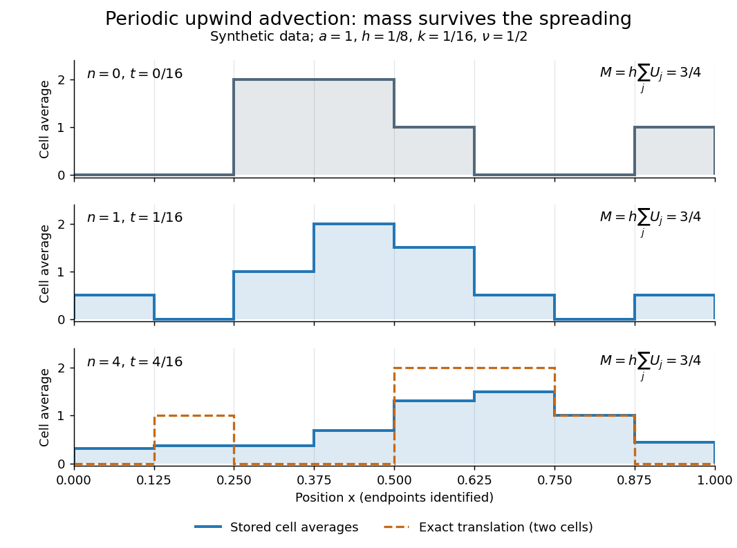
Original periodic upwind profile at zero, one and four steps: the integral remains three quarters while jumps spread
. Details. 
After four steps, , the exact translated profile has moved two cells to the right. Repeated averaging instead gives the explicit binomial coefficient formulawith all indices modulo eight. The diagram compares these computed cell averages with the exact translated cell averages. Their integrals agree, but the numerical jumps spread across cells. The finite volume method is useful for jump discontinuities because it retains the integral balance even at a jump; conservation alone does not guarantee a sharp profile. At this particular update is an exact one-cell shift, whereas for it mixes neighboring states. No accuracy conclusion at a jump follows just from the conserved total.
Articles by others on the same topic
There are currently no matching articles.