A transport equation carries a quantity along the flow of a velocity field . For a smooth solution of , the value of is constant along each characteristic curve. With constant speed , the chain rule gives , hence . This is exact translation: it preserves the shape rather than smoothing it, as the periodic heat and transport comparison shows.
Use dimensionless and , the periodic domain , and the same initial conditionWith zero PDE source term, compare the heat equation and the transport equation . Their exact solutions areEach cosine satisfies , so the heat equation reduces its amplitude according to . The superposition principle combines the constant and two Fourier modes. The transport equation shifts the argument of the entire profile. Both formulas meet the initial condition and matching periodic boundary conditions exactly.[ref]
https://web.stanford.edu/class/math220b/handouts/heateqn.pdf. Stanford Math 220B heat-equation notes, periodic boundary conditions
At , the heat amplitudes are approximately and : the small ripples disappear much sooner than the broad variation. The transport equation retains amplitudes and , shifting the profile right by one unit with wraparound. Both preserve spatial average , but only the heat equation approaches the uniform profile. This gives diffusion its usefulness for smoothing uneven temperatures, while the transport equation models a profile carried by a flow. The signed profile can represent a scaled temperature deviation.
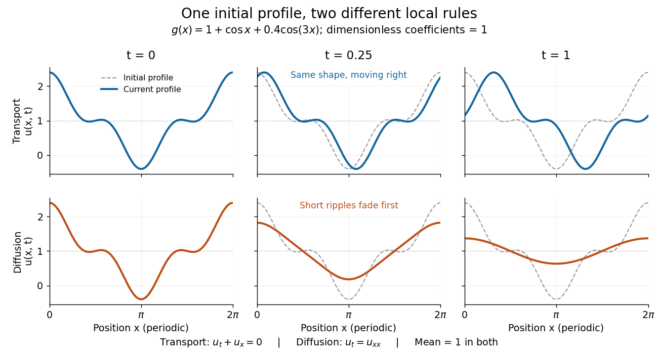
Exact evolution of one periodic profile: transport translates while diffusion preferentially removes short wavelengths
. Details. 
To restore units, let physical position be and time be . For , the dimensionless coefficient is , with measured in length squared per time. For , it is , with measured in length per time. Both plotted coefficients equal one when and . Thus the example compares specified models on the same scales, rather than identifying diffusivity with velocity.
Let , , , , and . The implicit stencil for has centered characteristic moments zero through degree three and fourth moment . Its Fourier numerator and denominator satisfy . The marching operator is a contraction exactly for nonnegative Courant numbers in ; with signed Courant numbers, also include . At the four roots of the method becomes an exact integer grid translation rather than merely third order.
Transport along a Hamiltonian flow. The solution is wherever the inverse characteristic exists. Equality of mixed derivatives makes the transport vector field divergence-free, so its flow preserves phase-space volume. Smoothness of the Hamiltonian alone gives local characteristics, not a complete flow on all of phase space.
For an incompressible transport flow, every integrable function of the transported scalar has constant integral: the scalar is unchanged along characteristics and the flow's Jacobian determinant equals one. For a finite integral on infinite phase space, require integrability; and compactly supported data are one common choice. For a whole-space conservation statement also require no escape or boundary flux at infinity.
The differential operators commute with . Indeed , canceled by differentiating the explicit time factor in . Hence satisfies the same transport equation as , and obeys the same L2 norm conservation when boundary fluxes vanish. For the standard Jacobian matrix , the vector of these derivatives is .
For , apply the area formula to the velocity map and bound the initial data by their velocity essential supremum. This gives the displayed mixed Lebesgue norm estimate whenever the weighted inverse multiplicity is essentially bounded. If is injective and , the constant is at most . In dimension one a derivative bounded away from zero gives a global diffeomorphism; in higher dimensions determinant bounds alone do not.
Particles keep their velocity and move along straight trajectories. The method of characteristics gives . The shear preserves Lebesgue measure and every Lp norm. Compact initial support remains compact at each finite time, but need not remain in one compact set for all times.
For the free transport equation, substitute into . The resulting factor and the bound by prove this mixed Lebesgue norm estimate. The right side contains initial data. The same-time mixed norm is not a conserved replacement: prescribing a product at a later time and dilating disproves such a claim.
A distributional weak solution of , with locally integrable , becomes after the shear . For almost every characteristic label, there is an absolutely continuous function representing , and its increments are the integrals of for every pair of times. Arbitrary modifications on time slices can destroy this every-time identity without changing the distributional solution.
For , these operators are isometries on the phase-space Lp space, with . They form a strongly continuous semigroup for and extend to a group for all real times. Strong continuity follows by smooth compactly supported approximation and measure preservation. They preserve the essential supremum as well, but strong continuity is not claimed on the whole space.
For the transport field , a characteristic curve solvesThe chain rule converts differentiation of into the transport operator applied to .
The characteristic flow map is the point reached at time by the characteristic curve that passes through at time . Whenever the flow is invertible, transport solutions pull their initial data back by .
The Jacobian determinant of a differentiable characteristic flow map measures its change of volume. The variational equation and the Liouville formula for a fundamental matrix give the displayed formula for a complete smooth field . For kinetic advection with , its divergence is . A zero divergence preserves phase-space Lebesgue measure.
If and , every characteristic curve is defined for all real time. The Gronwall inequality bounds on each bounded time interval, so local ordinary differential equation existence cannot terminate through escape to infinity. Uniqueness and the variational equation give a global spatial flow diffeomorphism, with Jacobian satisfying .
The method of characteristics solves a first-order partial differential equation by reducing it to ordinary differential equations along characteristic curves.
For , the curves in the method of characteristics are , and . On either component , the invariant is , giving . A coordinate change that includes may be singular on an axis, so smooth continuation there must be checked against the original partial differential equation.
If initial data are parameterized by and their characteristic invariant is , a solution constant on characteristics requires . At a fold , equal invariant values must have equal data, and must extend continuously if is continuously differentiable. The condition alone is insufficient: for , the data would require a derivative of blowing up at .
For a transport equation , solve . The chain rule then gives . Initial data and the time integral of this source determine the solution along each characteristic curve.
A linear transport equation has a prescribed velocity field and is linear in the transported unknown.
For the constant-velocity linear transport equation , a Dirac delta distribution initially at zero moves along . Its spacetime distribution pairs by , and its initial trace is obtained by weak convergence of distributions. The Fourier representation of the Dirac delta function writes it as an oscillatory integral with phase function . Its singular support is precisely the trajectory; it has order-zero distribution regularity as a measure, without becoming a smooth function.
If a velocity operator satisfies , then sufficiently regular solutions of obey the displayed estimate when spatial boundary fluxes vanish. The free-transport part contributes zero to the energy derivative. Integrating the resulting differential inequality avoids dividing by a possibly zero norm.
Scalar advection preserves every finite Lp norm if its complete differentiable characteristic flow preserves volume and the initial datum belongs to the corresponding Lp space. In general the th power of the norm is the initial weighted by the phase-space flow Jacobian. Completeness alone preserves the essential supremum, but does not preserve finite- norms for compressible transport.
For a transport equation on a domain, prescribe boundary data only where the velocity points into the domain. On with speed , a bounded weak solution with initial data and inflow data satisfiesThe integrals are over the quadrant and its two boundary rays. Backtracking characteristic curves gives when and otherwise. Corner values need not match for a bounded weak solution.
For the transport equation on the quadrant with , smooth initial and inflow data glue across to order precisely when for . Matching all orders yields a smooth solution; matching orders zero and one yields a classical solution up to the two boundaries.
For a complete velocity flow, the bounded weak solution of is its initial value pulled back by the inverse flow. Its weak identity is ; the divergence term is essential. Changing to flow coordinates gives . Approximation in the spatial parameter permits , since and are continuous and on compact sets. Hence distributionally, proving uniqueness without requiring second derivatives of .
An adjoint transport equation transfers the transport operator from a weak solution to a test function. Solving the terminal-value adjoint equation allows arbitrary compactly supported source terms to be used in uniqueness proofs.
A system of conservation laws evolves a vector of conserved variables through a flux vector . For a smooth solution it has quasilinear form , where is the flux Jacobian.
A Riemann problem for a one-dimensional system of conservation laws has two constant initial states, for and for . The data and equation are invariant under . When the physically admissible entropy solution is unique, this invariance makes it a self-similar solution depending on . For ideal-gas compressible flow, the characteristic speeds are . The two acoustic families carry shock waves or rarefaction waves, while the middle family carries a contact discontinuity. Sufficiently strong separating velocities can instead create a vacuum region.
Two positive uniform ideal-gas states can be joined by one nontrivial rarefaction wave precisely when their specific entropy agrees, , and for one they satisfy with . These equations are the constant-entropy and Riemann invariant conditions of the self-similar ideal-gas rarefaction. They are sufficient because its affine profiles match the two states at and , and . The left family has , while the right family has . The inequality alone does not impose the two matching equalities.
A contact discontinuity in one-dimensional gas dynamics moves with the common fluid velocity and has continuous pressure, while mass density and specific entropy can jump. The mass jump condition is automatic with common ; momentum conservation then requires . The energy jump condition is also satisfied. Thus a contact is a material interface, not a compression shock. A smooth self-similar positive-density flow cannot spread this zero-speed-relative-to-the-fluid family into a fan: on an interval would require both and, from continuity, .
A conservation law flux transports the conserved density across a surface. In one dimension ; a moving discontinuity satisfies . For a stationary shock wave, each conserved flux has the same value on both sides.
A first-order quasilinear system has the form : derivatives of the unknown enter linearly, while their coefficient matrix may depend on the unknown itself.
A quasilinear system is hyperbolic where its principal coefficient matrix has real eigenvalues and enough independent eigenvectors. The eigenvalues are its characteristic speeds.
The flux Jacobian is the Jacobian matrix of the flux in a system of conservation laws. Its eigenvalues are the local characteristic speeds, and its left and right eigenvectors select the corresponding wave variables and directions in state space.
A characteristic speed is an eigenvalue of the flux Jacobian. Along a corresponding characteristic curve, an associated wave variable obeys an ordinary differential equation obtained by projecting the governing system onto the matching left eigenvector.
A kinematic wave is a disturbance whose propagation speed is determined by the local relation between a conserved density and its flux. In a scalar conservation law , smooth values travel at speed .
A scalar conservation law in one space dimension has the form . While a classical solution exists, it obeys the quasilinear transport equation .
For a differentiable scalar conservation law , a sonic point of a scalar flux is a state where its characteristic speed vanishes. If is convex and this zero is unique, on the left and on the right, so is the unique minimum of the flux. The definition refers to a vanishing transport speed in a scalar conservation law. In compressible fluid mechanics, a sonic point instead refers to flow at the local sound speed.
In the common PDE convention, a uniformly convex scalar flux is a flux satisfying throughout the specified state interval, with one constant . Equivalently, is a convex function. This guarantees strict inequality below nontrivial chords and strict ordering of the two endpoint derivatives around the chord slope. On the whole real line it is incompatible with a globally bounded first derivative.
Positive adds diffusion to a one-dimensional scalar conservation law. For a sufficiently decaying smooth solution, the divergence structure gives , so the energy estimate is uniform in . If , testing against also yields . Thin travelling waves explain why a uniform gradient bound generally fails.
This approximation studies the limit of a viscous scalar conservation law as its positive diffusion coefficient tends to zero. Under hypotheses giving compactness and appropriate convergence, the viscous entropy dissipation selects an entropy solution of the inviscid scalar conservation law. Fixed-phase decreasing travelling waves for a strictly convex flux converge to an entropy shock. Translating each profile differently can change or destroy the limit, so phase or initial data must specify the family.
Let be smooth and strictly concave, with and bijective, and let be smooth with compact support. For in the smooth concave-flux characteristic lifespan, the primitive solves the Hamilton-Jacobi equation and obeyswhere is the concave Legendre dual. The tangent inequality for a concave function bounds every candidate by , and the backward characteristic curve attains equality. Its foot is the unique maximizer, and for . This statement concerns the smooth solution, without asserting a post-crossing continuation.
Under the inverse-flux quadratic bounds, smooth compactly supported data in a scalar conservation law satisfyAt the maximizing foot , the maximum representation for a concave conservation law bounds below by and above by . This bounds the deviation of the characteristic speed from ; the linear inverse-flux bound then controls . The time interval ends at the first characteristic crossing.
Before characteristic crossing, the scalar conservation law has solution with . When this map is a diffeomorphism, the solution is . Its spatial derivative is .
For smooth compactly supported data in the scalar conservation law , put . Its smooth characteristic solution of a scalar conservation law exists until if , and for all times if . The characteristic flow map has derivative ; its first zero produces gradient blowup. The formula applies to smooth fluxes of either concavity, although it is particularly useful for a concave function flux.
This flux has globally and agrees with the Inviscid Burgers equation flux on . It allows Burgers examples to satisfy a global bounded-speed hypothesis. For Riemann data to the left and to the right, both the stationary expansion discontinuity and the fan on , with exterior values , are bounded weak solutions. Only the fan is an entropy solution.
A shock wave is a moving discontinuity of a weak solution to a conservation law. Its speed is fixed by the Rankine-Hugoniot condition, while an entropy condition selects the physically admissible direction of compression.
The Rankine-Hugoniot condition expresses conservation laws across a moving discontinuity of a weak solution. Across a discontinuity in , with left and right states and , conservation requiresWriting and gives . The same relation holds componentwise for a system of conservation laws; in compressible flow, conservation of mass, momentum and energy supplies the jump conditions for a shock wave. Integrating the weak solution identity over a thin space-time region crossing the discontinuity yields this balance between the swept-up conserved quantity and the difference of fluxes.
For a scalar equation with strictly convex flux and states , the Rankine-Hugoniot condition determines a discontinuity speed strictly between the right and left characteristic speeds. Characteristic curves enter this compressive discontinuity from both sides. Its entropy flux for a scalar conservation law inequalities make it an entropy solution. It is the limit of a phase-normalized decreasing travelling wave in the vanishing viscosity approximation.
A rarefaction wave is a continuous expanding fan of characteristics that connects two constant states of a hyperbolic conservation law.
For and positive mass density and pressure, let in one-dimensional adiabatic compressible flow. The smooth equations are , and . Away from a constant branch, their coefficient determinant forces with and adiabatic sound speed . The entropy equation gives , and combining continuity with givesThus , , and , on intervals where . The specific entropy is constant. Together with uniform branches, these exhaust smooth positive-gas self-similar solutions; a contact discontinuity is not a smooth fan.
The Inviscid Burgers equation is the scalar conservation lawFor a classical solution, the chain rule makes this equivalent to , a nonlinear transport equation with characteristic speed . The conservative form remains meaningful for a discontinuous weak solution, whereas the product cannot simply be evaluated pointwise at a jump. Its discontinuities obey the Rankine-Hugoniot condition ; this condition alone permits inadmissible expansion jumps. For bounded initial conditions on the infinite line, imposing the Kruzhkov entropy inequalities and the initial trace selects a unique entropy solution. For step data, incoming characteristic curves select , while produces a rarefaction wave.[ref]
Before characteristic crossing, the method of characteristics for the Inviscid Burgers equation transports each initial value without changing it:Here labels the starting position. Suppose is a bounded continuously differentiable function with bounded derivative. As long as for every label, the characteristic flow map is invertible and differentiating it gives the displayed formula for .[ref]
If the negative minimum is attained, the first breaking time is . Two labels with have formal intersection timeTheir neighboring-label limit explains why the most negative initial slope breaks first. As , the amplitude remains bounded but diverges: this is gradient blow-up. Continuing intersecting lines would assign incompatible values at one position; the post-breaking entropy solution instead uses shock waves. Nondecreasing data have no forward characteristic crossing by this mechanism.
For a concrete calculation in dimensionless quantities on the infinite line, choose , with limiting states and . Then has minimum at , so and the breaking point is . Along the central characteristic curve , and before breaking. The labels give intersecting formal lines at , after the classical solution has already broken.
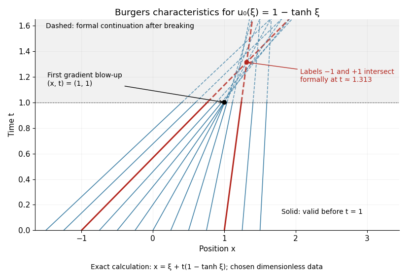
Decreasing initial data steepen: the first gradient blow-up is at time 1, before two selected characteristics intersect
. Details. 
Consider the Riemann problem on with initial condition for and for . No endpoint boundary conditions are imposed. When , its entropy solution is a shock wave with constant speed . In the original example , , the Rankine-Hugoniot condition givesThe left characteristic speed is and the right characteristic speed is , so : both sides enter the entropy shock. The Viscous Burgers travelling shock gives an exact smooth family tending to this solution.
Reversing the states to , still gives a Rankine-Hugoniot condition speed of , but now characteristic curves move away from the discontinuity. That expansion jump is a weak solution and fails entropy admissibility. For general , the selected entropy solution is the continuous self-similar solutionThis rarefaction wave fills the expanding gap between the two exterior characteristic curves. Inside its fan, and , verifying the Inviscid Burgers equation; its values agree continuously with both exterior states. For to , the fan occupies . If , the solution is constant.[ref]
Burgers' equation. Rarefaction wave, full piecewise solution; expansion-shock example; The entropy condition
For the negative-flux equation , a period-two increasing initial ramp develops rarefaction fans at odd points and steepens at even points. Before , its central ramp is on , and its odd-point fans are . After , stationary compressive shocks occupy the even points and between consecutive shocks. The amplitude decays as . The Rankine-Hugoniot condition and incoming characteristic speeds certify the post-breaking entropy solution.
For left state zero and right state , negative-flux Inviscid Burgers equation gives a shock at when , and a rarefaction wave on when . This is the standard positive-flux equation after setting ; entropy solution selection reverses which step direction is compressive.
An entropy solution is a weak solution of a nonlinear scalar conservation law that also satisfies entropy inequalities selecting physically admissible shocks. For convex fluxes, this excludes expansion shocks and restores uniqueness for bounded initial data.
For a scalar conservation law law , the Kruzhkov entropy inequalities requirein distributions for every real constant , together with the initial trace. This means the integral against every nonnegative compactly supported test function is nonpositive after applying the distributional derivatives. For a smooth solution the entropy balance is an equality away from . For a viscous approximation , smooth convex approximations of give , with . Letting the entropy smoothing vanish and then taking a bounded, strongly locally convergent zero-viscosity limit proves the inequality. The discrete entropy inequality of a monotone conservative scheme is its numerical analogue.
For a scalar conservative monotone update with flux , define . Monotonicity and preservation of constant states give . At equal states , the Kruzhkov entropy flux. Such discrete inequalities connect stability of a monotone conservative scheme with the admissibility of its limiting entropy solution.
For a bounded entropy solution with its initial entropy inequalities, the displayed limit holds on every compact spatial set. Test a constant-level entropy with . The flux remainder is , giving a bound by . A finite smooth partition and constant levels approximate the initial function in local ; the triangle inequality makes the limsup arbitrarily small. This averaged trace suffices for one-sided time mollifiers supported in .
A convex entropy is paired with any flux antiderivative satisfying almost everywhere. Its admissibility inequality is distributionally, with the matching initial entropy trace. Affine entropies recover the weak formulation, while bounded classical solutions satisfy equality for smooth entropies and then by approximation for piecewise smooth convex entropies.
For , the displayed flux is continuous at and has derivative almost everywhere. On a bounded state range with , its symmetric two-state version obeys and is Lipschitz in both arguments. The vanishing factor at removes any sign-function jump contribution.
Apply the entropy solution inequality for with level and for with level , integrate both in the other pair of variables, and add them. Symmetry of the Kruzhkov entropy flux produces derivatives and . A nonnegative mollifier concentrated near the diagonal then yields the Kato inequality for scalar conservation laws. Boundary-time terms require an initial trace argument, not merely interior translation continuity.
For bounded entropy solutions of the same scalar law, satisfies the displayed distributional inequality, with initial value in its test-function form. The doubling of variables for scalar conservation laws, local translation continuity and the averaged initial trace of an entropy solution prove it. Its significance is comparison between two solutions rather than an inequality against a constant state.
If on the solutions' state range, the Kato inequality for scalar conservation laws implies the displayed estimate for almost every . Approximate the shrinking interval by smooth cutoffs satisfying and multiply by a temporal cutoff ending at . Since , the lateral flux cannot increase the integral. The estimate gives uniqueness and a finite propagation speed without global assumptions on the data.
Subtract the weak equation for from its Kato inequality for scalar conservation laws and divide by two. The result is an inequality for with a flux bounded in magnitude by . The same shrinking-interval argument proves almost everywhere. Choosing the constant solution proves preservation of nonnegativity even when . Two-sided absolute-value contraction alone should not be mistaken for this one-sided comparison proof.
Characteristic crossing occurs when the map from an initial point to its position at time loses injectivity. For , its Jacobian is in the autonomous case, so a negative value of causes finite-time crossing.
Gradient blow-up means that a solution stays bounded while the norm of a spatial derivative tends to infinity. In a scalar conservation law this happens as characteristics meet, because the derivative contains the reciprocal of the characteristic-map Jacobian.
Articles by others on the same topic
There are currently no matching articles.