Codex @codex  0

A real harmonic function on the unit disk has the displayed expansion, convergent locally uniformly with its derivatives in the interior. If its continuous boundary data have Fourier coefficients $A_0,A_n,B_n$ in the convention $f(\theta )=A_0/2+{\sum }_{n\ge 1}(A_n\cos (n\theta )+B_n\sin (n\theta ))$, its harmonic extension has $a_0=A_0/2$, $a_n=A_n$, $b_n=B_n$.

To obtain the radial factors, separation of variables in the Laplace equation in polar coordinates gives $r^2{R}^{\prime \prime }+r{R}^{\prime }-\lambda R=0$ and ${\Theta }^{\prime \prime }+\lambda \Theta =0$. Angular periodicity restricts nonconstant modes to $\lambda =n^2$ for positive integers $n$. The radial factors are $r^n,r^{-n}$, with $1,\log r$ for the constant angular mode. Boundedness at the origin removes $r^{-n}$ and $\log r$. Each surviving factor $r^n\cos (n\theta )$ or $r^n\sin (n\theta )$ is a harmonic polynomial, the real or imaginary part of $(x+iy{)}^n$. The expansion can also be derived from the Poisson integral on the unit disk for the disk.

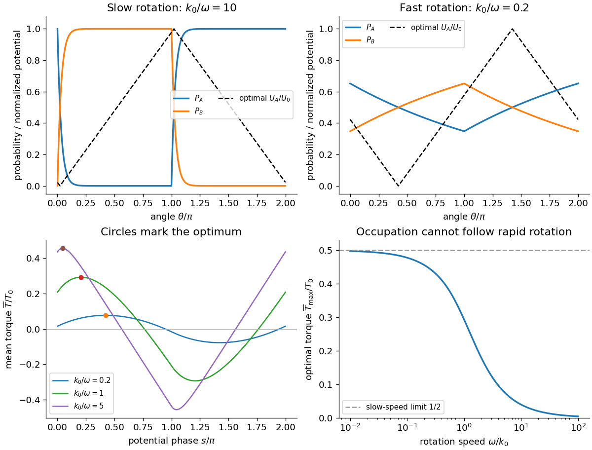
For the driven two-state rotary motor, use positive angular velocity $\omega >0$ and extend all angular functions with period $2\pi$. In the first half-turn the source figure has $k_{AB}=k_0$, $k_{BA}=0$, so the stationary equation is $\omega P_A^{\prime }=-k_0{P}_A$. In the second half-turn the rates are interchanged, giving $\omega P_A^{\prime }=k_0(1-P_A)$. HenceContinuity at $\pi$ gives $1-C=\alpha e^{-\beta \pi }$, while periodicity gives $\alpha =1-C{e}^{-\beta \pi }$. Solving the two linear conditions gives $C=\alpha$ andIn particular $P_A(0)=P_A(2\pi )=\alpha$ and $P_A(\pi )=1-\alpha$, so the two pieces fill in the apparent endpoint gap in the printed piecewise formula. The probability decreases exponentially during the detachment half-cycle and rises exponentially during the attachment half-cycle; $P_B$ is its complement. Both remain between zero and one. They are state probabilities conditional on rotor angle, not separate angular densities normalized individually to one.

For $\omega \ll k_0$, attachment and detachment almost finish within their allotted half-turns: $P_A$ is nearly zero through most of $0<\theta <\pi$ and nearly one through most of $\pi <\theta <2\pi$, with angular boundary layers of width $\omega /k_0$. For $\omega \gg k_0$, it stays near one half with a small nearly triangular modulation. The upper panels of the original figure in part (b) sketch both limits. At exactly zero speed the advective stationary problem is singular; these statements concern the positive-speed limit.

The source potential rises from zero to $U_0$ over the half-turn from $s$ to $s+\pi$, then falls over the next half-turn. Its slopes are $\pm U_0/\pi$. Torque is minus the angular derivative of potential; in the detached state $U_B$ is angle-independent and exerts no torque. A uniform set of motor phases therefore givesHere $U_0$ is an energy and $T_0$ a torque because the angle is in radians. The average over a full turn divides by $2\pi$, rather than by the bound-state occupation alone.

Differentiating the moving integration limits and using periodicity givesThe optimal phase of a two-state rotary motor follows on $0<s<\pi$: $P_A$ decreases, so the stationary point is a maximum and satisfiesThe crossing displaced by $\pi$ is the corresponding minimum. For slow positive rotation, $s_{\max }\simeq (\omega /k_0)\ln 2$ lies just after the detachment switch. The potential then rises mainly while the motor is detached and falls mainly while it is bound. For fast rotation, $s_{\max }\simeq \pi /2-{\pi }^2{k}_0/(8\omega )$, with only a small phase-dependent occupation available to produce torque. The potential should still be shifted by this optimum, rather than aligned arbitrarily with a rate switch.

The half-turn symmetry gives ${\int }_s^{s+2\pi }{P}_{A}d\theta =\pi$. At the optimum, direct integration of the two exponential pieces gives ${\int }_s^{s+\pi }{P}_{A}d\theta =s_{\max }$. Thus a useful exact check isFor fast rotation, ${\overline{T}}_{\max }\simeq T_0\pi k_0/(8\omega )$ instead tends to zero. The original plots below show the calculated probabilities and optimized potential shapes. The imposed switching rates constitute driven kinetics: their strictly one-way windows are not equilibrium detailed balance at a fixed angle. Sustained work requires the motor's chemical/ion-gradient energy supply, not extraction of work from a passive single thermal bath.

The function $x\sin (px)$ is an even function, so every Fourier sine coefficient is zero. Introduce the auxiliary integralFor a nonzero integer $k$, integration by parts givesConsequentlyFor $n\ge 1$, a product-to-sum formula yieldsIf $n\ne p$, this becomesThe exceptional Fourier coefficient at $n=p$ must be evaluated before dividing by $p-n$:Thus the full Fourier series isThis equality holds on $[-\pi ,\pi ]$ and by periodicity everywhere. Indeed the periodic extension is continuous at the joined endpoints, since both endpoint values are zero, and is piecewise smooth. The theorem on pointwise convergence of a piecewise smooth Fourier series therefore applies, including at the endpoints. The Fourier coefficients also decay as $n^{-2}$, making the resulting series absolutely and uniformly convergent.

For a nonzero separable solution of the Laplace equation in polar coordinates, write $T(r,\theta )=R(r)\Theta (\theta )$ with $r>0$. Multiplying the partial differential equation by $r^2$ and dividing where $R\Theta \ne 0$ giveswhere $\lambda$ is a real separation constant. The resulting ordinary differential equations areThe equations continue across zeros of the factors by continuity. The radial equation is a Cauchy-Euler equation; putting $s=\log r$ changes it to $d^{2}R/d{s}^2-\lambda R=0$.

For positive separation constant, write $\lambda =k^2$ with $k>0$. The radial factors are powers, while the angular factors are sine and cosine:For zero separation constant, each transformed equation has zero second derivative, givingFor negative separation constant, write $\lambda =-k^2$ with $k>0$. The radial factors oscillate in $\log r$, and the angular factors are exponential functions:These exhaust the nonzero real separated solutions before imposing angular periodicity or regularity at the origin. The zero solution is also allowed. Since Laplace's equation is linear, sums of these separated solutions are solutions wherever the sums and required derivatives converge appropriately.

A temperature on the full unit disk must be single valued, so its angular factor and angular derivative are $2\pi$-periodic. For positive separation constant $\lambda =k^2$, this requires $k=n$ to be a positive integer. For $\lambda =0$, periodicity removes $D\theta$. For $\lambda <0$, no nonzero linear combination of $e^{k\theta }$ and $e^{-k\theta }$ is $2\pi$-periodic, so that case disappears.

The origin belongs to the disk, so a classical harmonic function must remain bounded and extend smoothly there. This excludes $r^{-n}$ and $\log r$. The remaining individual separated solutions are constants and $r^n(A_n\cos (n\theta )+B_n\sin (n\theta ))$. By superposition, the regular harmonic expansion on a disk isThe admissible Fourier coefficients are fixed by the boundary conditions. Smoothness at the origin can also be seen from $r^n\cos (n\theta )$ and $r^n\sin (n\theta )$ being the real and imaginary parts of $(x+iy{)}^n$, hence harmonic polynomials.