A point process records random locations by a random measure that counts them. Examples include arrival times of a queue, positions of stars, and the finite eigenvalue configuration of a random matrix. The count in an observation window is a random variable; its expected value is supplied by the intensity measure of a point process, while its fluctuations and relationships with other windows require more information.
For a precise spatial convention, take with its Borel sigma-algebra and a probability space . A locally finite point process is a measurable function from to the space of locally finite point measures, equipped with the sigma-algebra generated by evaluations for Borel sets . Each realization has the formwhere is finite or countable and repeated locations are allowed; is a Dirac measure. Here a point measure is a counting measure with possible multiplicities, rather than the counting measure of a set of distinct locations.[ref]
Lectures on the Poisson Process by Günter Last and others. Section 2.1, Definition 2.1, printed pp. 10-11: point measures and the sigma-algebra generated by evaluations
Local finiteness means for every bounded Borel set , on a single almost sure event. In it suffices to check the countable collection of balls of integer radius centered at the origin, and this is equivalent to finiteness on every compact set. On a general measurable space there is no notion of boundedness without additional structure: state a metric or an explicit family of observation windows. Another convention on locally compact spaces requires finiteness on compact sets; this need not coincide with finiteness on all bounded sets outside . Local finiteness does not require finitely many points in all of .[ref]
Lectures on the Poisson Process by Günter Last and others. Section 2.4, Definitions 2.11 and 2.13, printed pp. 16-17: bounded-set local finiteness and the countable ball exhaustion
A point process is simple when, on a single almost sure event, every location has multiplicity at most one. Its realizations are simple locally finite point measures. For instance, is locally finite but not simple: it has four points counted with multiplicity at three distinct locations. Simplicity is a statement about each entire realization. Checking separately for every fixed is insufficient: with having the uniform distribution on passes every such fixed-location check, yet always has a double point.[ref]
Lectures on the Poisson Process by Günter Last and others. Section 6.2, Definitions 6.6 and 6.8, printed p. 49: simple measures and simple point processes
For a bounded Borel set , the window count of a locally finite point process is a finite nonnegative integer random variable. It counts multiplicities, and the convention for window boundaries matters. On the time half-line, is a counting process and . For pairwise disjoint observation windows , the measure identityis valid for every realization. Additivity of counts supplies no independence assumption.
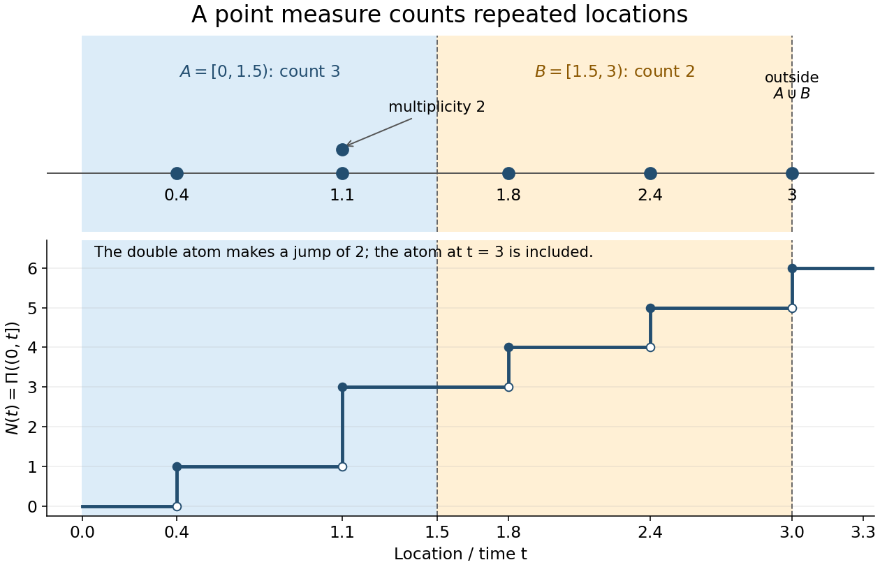
Window counts include multiplicity and depend on boundary conventions
. One locally finite point measure is . The half-open windows and have counts three and two; . The atom at three lies outside both windows. Two stacked dots denote the double atom at , and the step plot records , which includes the atom at three. Details.
Observation windows are measurable sets used to count points of a point process. They are pairwise disjoint when for every . Half-open intervals such as and meet at a boundary without sharing any point, whereas the closed intervals and both contain one. A disjoint union makes window counts additive; it does not make their random variables independent.
A point process on is stationary if every translation preserves its probability law. If its mean count in a unit cube is finite, its intensity measure is for some , where denotes Lebesgue measure. This follows because stationarity makes the mean measure invariant under translations. A constant intensity function of a point process describes only these mean counts, and by itself asserts neither stationarity of the entire law nor independence.[ref]
Lectures on the Poisson Process by Günter Last and others. Section 8.1, Proposition 8.2, printed pp. 69-70: stationarity and constant intensity under a finite unit-cube mean
A Neyman-Scott process places independent offspring clusters around points of a Poisson parent process, with an independently drawn offspring count and displacements. Poisson offspring counts make the offspring process conditionally Poisson given the parents, and therefore give a Cox process. Arbitrary offspring counts need not have that property.
The intensity measure of a point process is its expected counting measure:It may take the value .[ref]
Lectures on the Poisson Process by Günter Last and others. Section 2.2, Definition 2.5, printed p. 12: intensity as the expected counting measure
Countable additivity follows by applying the monotone convergence theorem to the counts of finite unions of pairwise disjoint observation windows. If is locally finite and absolutely continuous with respect to Lebesgue measure, its Radon-Nikodym derivative is the intensity function of a point process :This is an expected number per unit volume, not a probability density function for a randomly selected point. For example, a single deterministic point has , a Dirac measure, and no Lebesgue measure density. The density representation requires its own assumption.[ref]Spatial Point Processes and their Applications. Section 2.1, Definitions 2.1-2.2, printed pp. 26-27: expected counts and intensity functions
For a bounded Borel set , , but local finiteness alone does not ensure that this expected value is finite. Conversely, implies almost surely, even when is unbounded. A constant finite intensity function of a point process on all of has infinite total intensity measure, although every bounded window has finite expected value.
Here is an explicit example even within simple point processes. Let be a positive integer with probability mass function . The telescoping series sums to one, is finite almost surely, but . Conditional on , sample independent points with the uniform distribution on . The resulting point process has finitely many distinct points almost surely, while . Thus finite counts in each realization and finite mean counts are separate requirements; local finiteness of the intensity measure is an integrability assumption.
The same intensity measure can belong to very different point processes. A Poisson point process with a locally finite intensity measure adds two requirements: each finite-intensity window count has the Poisson distribution of mean , and counts in pairwise disjoint observation windows are mutually independent. These requirements determine its probability law; they do not follow from the formula for .[ref]
Lectures on the Poisson Process by Günter Last and others. Section 3.1, Definition 3.1 and Proposition 3.2, printed pp. 19-20: Poisson count laws, independence, and uniqueness
A randomly shifted lattice point process, a unit-rate Poisson point process, and the shared random rate gives dependent point counts construction all satisfy on the real line. Nevertheless, their counts in have respectively variance zero, one, and two. Counts in the disjoint observation windows and have respectively covariance , zero, and . These exact calculations show why measuring mean density cannot identify a spacing or statistical dependence model.
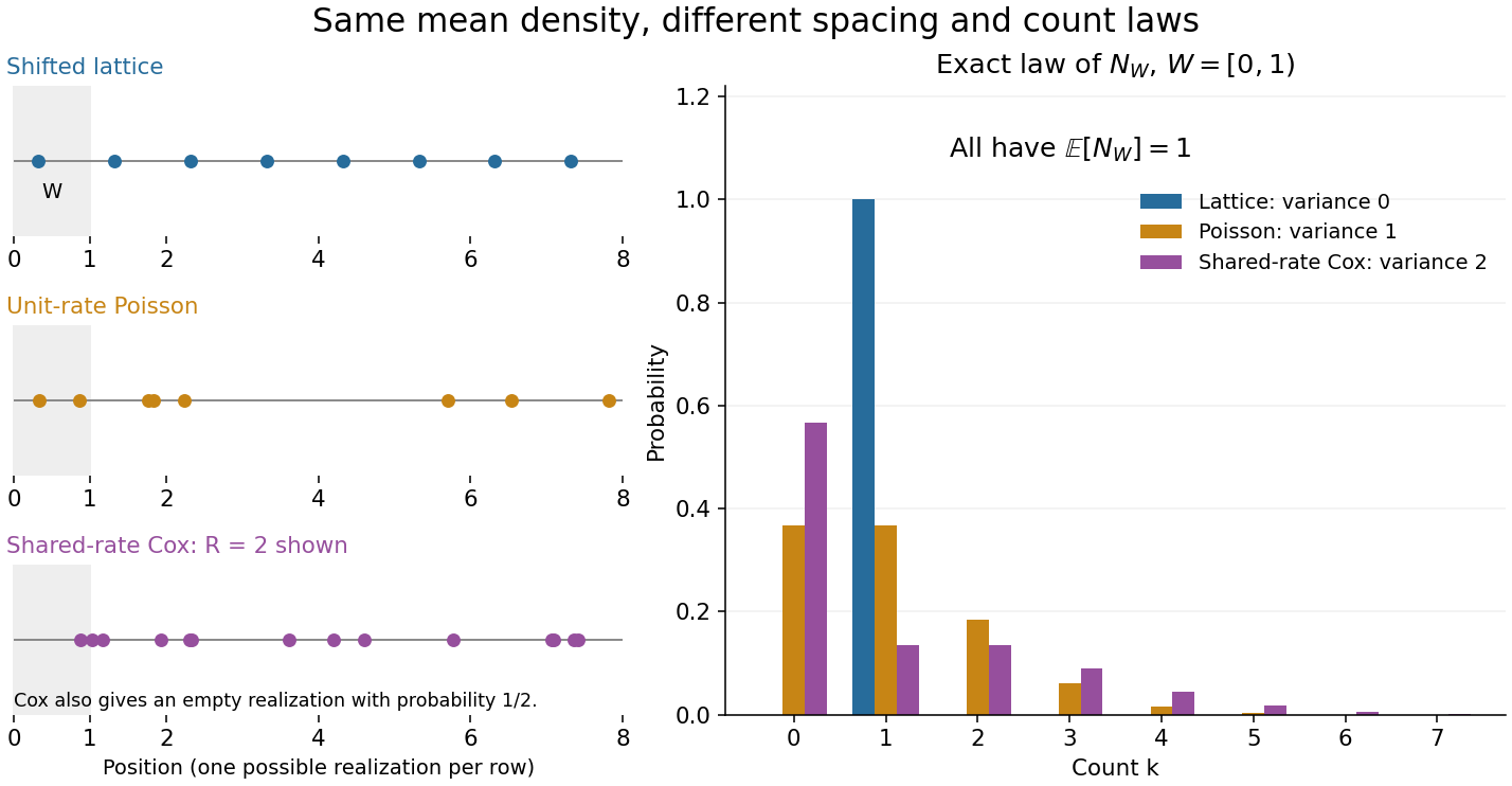
Equal intensity permits regular spacing, Poisson counts, and shared-rate dependence
. All three laws have intensity measure . Left: illustrative realizations of a randomly shifted lattice point process, a unit-rate Poisson point process, and the shared random rate gives dependent point counts construction conditional on rate two; the latter also has a completely empty outcome with probability . Right: exact probability mass functions of the count in , with the axis displayed through seven. Equal expected values of one coexist with variances zero, one, and two. Realizations illustrate spacing; the bars describe laws, not frequencies estimated from those realizations. Details.
Let have the uniform distribution on and place a point at every , . This is a simple point process, locally finite, and a stationary point process: a translation only changes the phase modulo one, preserving its uniform distribution. For every Borel set , the Tonelli theorem givesIts consecutive points are exactly one unit apart, despite having the same intensity measure as a unit-rate Poisson point process. This is the one-dimensional translated-grid construction.[ref]
Spatial Point Processes and their Applications. Section 2.1, Example 2.3, printed pp. 26-27: randomly translated grids have constant intensity
Every half-open interval of length one contains exactly one point. For and , , each count has the Bernoulli distribution with parameter , andMore generally, an interval of length , with a nonnegative integer and , contains or points with probabilities and . Its count variance is , while a unit-rate Poisson point process has count variance .
The void probability functional assigns to a measurable set the probability that it contains no atom of a random point measure. For a Poisson random measure of intensity , it is . The exponential void probabilities characterize a Poisson random measure result uses simplicity; doubling every atom of a Poisson measure preserves void probabilities but changes count distributions.
If bounded intervals have void probabilities for Lebesgue measure , a fixed deterministic point has zero chance of being an atom. Surround it by intervals of lengths tending to zero and use . This holds for each fixed endpoint, not simultaneously for all real points of a nonempty point process.
A point measure is a countable sum of Dirac measures. It is simple if all its atoms have mass one, and locally finite if every bounded set has finite mass. Simplicity lets fine enough cells count individual points, whereas occupation indicators would lose multiplicities in a nonsimple measure.
For a fixed bounded interval with no atoms at its endpoints, the occupation count of fully contained half-open dyadic intervals increases to the true count of a simple locally finite point measure. Refinement cannot reduce occupancy. Finitely many distinct atoms in a bounding interval have positive minimum separation; for fine enough cells each atom lies alone, and every interior atom's cell is contained in the target interval. Thus the counts eventually agree, path by path.
A point process is determinantal with kernel relative to a specified reference measure if every correlation function of a point process is the indicated determinant. A rank- finite-rank projection kernel gives an exactly -point process, whose symmetric joint density is .
The th correlation function is the density of the th factorial moment measure: integrating a nonnegative test function against gives the expectation of its sum over ordered -tuples of distinct points. For exactly exchangeably labelled points with symmetric joint density , it is times the marginal density of labels. It is not normalized to have total mass one.
Articles by others on the same topic
There are currently no matching articles.