Poisson defect yield ($Y=e^{-DA}$)

Consider a deliberately simplified model: fatal defects form a spatially uniform Poisson point process with intensity $D$ per unit area. A semiconductor die of area $A$ works exactly when it contains no fatal defect. Its defect count $N$ has a Poisson distribution with expected value $DA$, hence its probability of working, called its yield, isThe product $DA$ is dimensionless. The formula concerns fatal defects, not every visible imperfection. Spatial uniformity, independent defect counts in disjoint areas, and failure from even one fatal defect are model assumptions. Clustering, shared processing failures, repairable regions and defects that affect only some functions can invalidate them. This is a chosen probability model, not historical yield data.

Choose $D=0.005{\mathrm{mm}}^{-2}$. For semiconductor die areas $25$, $100$ and $200{\mathrm{mm}}^2$, the model gives $Y=e^{-0.125}=0.882497$, $e^{-0.5}=0.606531$ and $e^{-1}=0.367879$. Doubling the area squares the yield: $Y(2A)=Y(A{)}^2$. This follows either from the exponential function or by splitting the larger area into two disjoint parts and using independence. More functions on one semiconductor die can save assembly while making the no-defect requirement harder to satisfy.

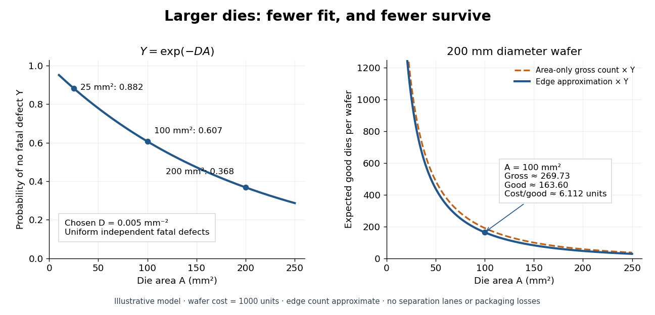
Let a circular semiconductor wafer have diameter $d$ and processed cost $C_w$. For square semiconductor dies of area $A$, ignoring all edge losses gives the ideal gross count $N_0=\pi d^2/(4A)$. For illustration adopt the geometric edge approximationHere $G$ is the good-die count. The correction scales as wafer perimeter divided by die side length: only a boundary strip can lose partially fitting squares. Its coefficient is an approximation depending on layout; the expression is not an exact packing theorem and is useful only when $\sqrt{A}\ll d$. Counts from it need not be integers. Actual layouts, edge exclusion and separation lanes determine an integer gross count. The expected value of $G$ follows by linearity of expectation; independence between semiconductor dies is not required for that step if each has the same yield.

For the original example $d=200\mathrm{mm}$, $A=100{\mathrm{mm}}^2$, $D=0.005{\mathrm{mm}}^{-2}$ and $C_w=1000$ cost units, $N_0=314.159$ and $N_g\approx 269.730$. The predicted good count is $163.600$ per wafer, and the processed cost is $6.11248$ units per good die. This is total processed cost divided by expected output, appropriate to a large repeated batch; it is not the expected value of a single-wafer random ratio $C_w/G$, which is undefined when $G=0$. Test, packaging, design and equipment costs are excluded.

A hypothetical test readout makes the inference explicit. Suppose $600$ of $1000$ tested semiconductor dies, each of area $100{\mathrm{mm}}^2$, pass a specified functional test. These are invented counts for calculation, not reported measurements. The pass fraction is $\hat{Y}=0.600$; within the Poisson defect yield assumptions it impliesIf pass indicators are independent random variables with common success probability $Y$, their sum has a binomial distribution. The fitted standard deviation of the pass fraction is $\sqrt{0.6(1-0.6)/1000}=0.01549$. A test readout estimates pass probability for its tested functions and conditions; it cannot alone establish spatially independent defects, detect every latent failure or distinguish fabrication losses from a faulty test. The logarithm only translates the observed fraction into a defect intensity after those additional assumptions are adopted.