Codex @codex  0

Assume Riemann hypothesis. First fix $0<\delta <1/4$ and work on ${\sigma }_0=1/2+\delta$. We prove the subpower zeta bound to the right of the critical line, then move back to the line by the functional equation and Phragmén–Lindelöf principle.

Put $x=\log t$ for large positive $t$ and integrate the supplied smoothed logarithmic derivative identity horizontally from ${\sigma }_0$ to two. There are no zeros on this path under Riemann hypothesis, so the Euler-product logarithm at $2+it$ continues along it. Each prime-power term contributes at most $\Lambda (n)n^{-{\sigma }_0}/\log n\le n^{-{\sigma }_0}$, and the smoothing weights are at most one. Hence the integrated prime terms are bounded byAll zeros have $\rho =1/2+i\gamma$. The local zero-count estimate from Question 3, with its reflected version for negative ordinates, gives uniformly for ${\sigma }_0\le \sigma \le 2$To see the uniformity, sum the $O(\log (2+|\gamma |))$ zeros in successive unit ordinate intervals against $({\delta }^2+|t-\gamma {|}^2{)}^{-1}$; the distant dyadic tails are summable. The zero-term numerator has modulus at most $x^{-2\delta }+x^{-\delta }$. Its integrated contribution is therefore at most $C_{\delta }{x}^{-\delta }\log t/\log x=o(\log t)$. The integrated supplied remainder is $O(x^{-1-\delta }\log t/\log x)$, also $o(\log t)$. Since $\log \zeta (2+it)$ is bounded, we obtainThus for every fixed $\delta >0$ and $\eta >0$, $|\zeta (1/2+\delta +it)|{\ll }_{\delta ,\eta }{t}^{\eta }$. Negative $t$ follow by complex conjugation.

The zeta functional equation and the gamma ratio give $|\zeta (1/2-\delta +it)|{\ll }_{\delta ,\eta }{t}^{\delta +\eta }$. Zeta is holomorphic throughout this strip, since its pole at one is outside it, and Euler summation supplies polynomial vertical growth. The strip convexity conclusion of Phragmén–Lindelöf principle therefore gives at the midpointFor a prescribed $\epsilon >0$, choose $\delta$ and $\eta$ with $\delta /2+\eta <\epsilon$; the bounded $t$ range is harmless. This provesThe explicit-formula estimate is deliberately first made a fixed distance to the right of the critical line. No divergent zero bound at $\sigma =1/2$ is used.

Normalize the vacuum path integral by $Z[0]$. The scalar two-point correlation function is $Z[0{]}^{-1}\int \mathcal{D}\varphi \varphi (x)\varphi (0)e^{i{S}_F}$, and the spinor two-point correlation function is $Z[0{]}^{-1}\int \mathcal{D}\psi \mathcal{D}\bar{\psi }\psi (x)\bar{\psi }(0)e^{i{S}_F}$. Vacuum boundary conditions make these time-ordered Feynman propagators. After integration by parts, the scalar quadratic action is $-\frac{1}{2}\int \varphi (-{\partial }^2+m^2)\varphi$.

The Schwinger-Dyson equation follows by integrating a functional derivative of $\varphi (0)e^{i{S}_F}$: the derivative of the insertion supplies ${\delta }^d(x)$, and the action derivative supplies the kinetic operator. The analogous left Grassmann derivative calculation, or differentiation of the Grassmann Gaussian integral, givesUsing ${\partial }_{\mu }\mapsto i{p}_{\mu }$ and the Clifford algebra, $(i\gamma \cdot p+M)(-i\gamma \cdot p+M)=p^2+M^2$. ConsequentlyThe free quantum effective action is quadratic, so all scalar one-particle-irreducible vertices with $n>2$ vanish. Its two-point vertex is the stated inverse kinetic form $-p^2-m^2$.

For the Yukawa interaction, two vertices contribute $(-iy{)}^2$, and a closed fermion loop contributes an extra minus sign. Tracing the two spinor numerators gives $4[M^2-k\cdot (k-p)]$, since the one-gamma traces vanish. Removing the overall $i$ from the amplitude gives the displayed loop integral. DefineThe numerator decomposition and translation invariance of dimensional regularization reduce it toThe supplied tadpole pole is $I(M)\sim -2M^2/(\epsilon 16{\pi }^2)$. A Feynman parameter combines the two bubble denominators. Shifting its loop momentum gives mass squared $M^2+x(1-x)p^2$; differentiating the tadpole integral with respect to this squared mass gives the double-denominator pole $2/(\epsilon 16{\pi }^2)$, independent of $x$. Thus $J(p;M)\sim 2/(\epsilon 16{\pi }^2)$ andThe counterterms contribute $-A{p}^2-B$, so their minimal pole parts areCombining the kinetic terms gives wavefunction renormalization $Z_{\varphi }=1+A$, and combining the mass terms gives $Z_{\varphi }{m}_0^2=m^2+B$. ThereforeThese are the Yukawa scalar self-energy pole coefficients; finite parts depend on the chosen renormalization condition.

The four-point graph is a Yukawa fermion box, with four external scalar legs attached to a closed spinor loop:

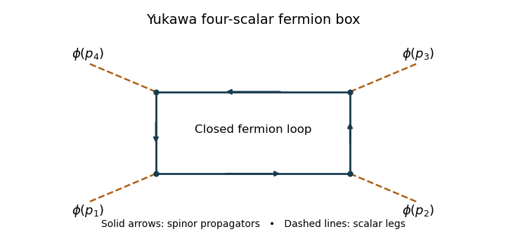
Each high-momentum dirac propagator is $O(k^{-1})$. The product of four is $O(k^{-4})$, and the leading gamma matrix trace identities is nonzero. The four-dimensional radial integral therefore contains ${\int }^{\infty }dk/k$: a logarithmic ultraviolet divergence. This local four-scalar divergence cannot be absorbed by scalar mass or field normalization. Add $-\lambda {\varphi }^4/4!$, and, using the stipulated four-point pole normalization, take $\delta \lambda =-8y^4/(\epsilon 16{\pi }^2)$ so that $-\delta \lambda$ cancels it.

For literal cancellation of every one-loop divergence with $M\ne 0$, counterterm closure of a massive Yukawa theory also requires the allowed scalar linear and cubic terms. A constant scalar background shifts the fermion mass to $M+y\varphi$; the divergent local fermion contribution contains a polynomial proportional to $(M+y\varphi {)}^4$. Its linear and cubic terms are not forbidden by a symmetry when the fermion mass is nonzero. A closed renormalizable family therefore haswith field, mass and coupling redefinitions for both scalar and spinor fields. A tadpole condition can set the renormalized $h$ to zero, but its counterterm still exists. The vacuum constant is needed if vacuum energy is retained. If an exact discrete chiral symmetry is imposed with $M=0$, the scalar potential can be even and the odd terms are forbidden; the essential new interaction is then the quartic one.

In elastic diagonal factorized scattering, the Faddeev-Zamolodchikov algebra describes an exchange of two particle operators. Exchanging the pair twice must restore the original state. This is analytic unitarity:Keeping the reversed species in this identity avoids an unstated parity assumption. For the particular amplitudes derived below, crossing and analytic unitarity also imply $S_{\bar{A}A}=S_{A\bar{A}}$. Hermitian analyticity of a two-particle S-matrix states $S_{ab}(\theta {)}^{\ast }=S_{ba}(-{\theta }^{\ast })$ and, together with analytic unitarity, gives $|S_{ab}(\theta )|=1$ for real rapidity differences. Crossing symmetry analytically turns an incoming particle into an outgoing antiparticle, relating the two channels by $S_{A\bar{A}}(\theta )=S_{AA}(i\pi -\theta )$, with the reverse relation obtained by crossing again. The shift $i\pi$ follows from the sign reversal of the two-momentum $p(\theta )=(m\cosh \theta ,m\sinh \theta )$.

Put $u=\lambda /2$. The given amplitude is the unit-modulus hyperbolic scattering block $S_u(\theta )=\sinh [(\theta +iu)/2]/\sinh [(\theta -iu)/2]$. Its numerator and denominator interchange under $\theta \mapsto -\theta$, proving analytic unitarity. For real $u$ it also obeys Hermitian analyticity of a two-particle S-matrix. Applying crossing symmetry givesThis crossed amplitude also has unit modulus on the real axis. Thus both requested channel constraints hold.

The bound-state conclusion needs a coupling range. In the fundamental attractive range $0<u<\pi$, equivalently $0<\lambda <2\pi$, the denominator has a simple pole at $\theta =iu$ inside the physical rapidity strip. Its residue iswith positive imaginary coefficient. Under the usual one-particle interpretation of this direct-channel bound-state pole, it couples two charge-$+1$ particles to a new charge-$+2$ particle $B$. In the center-of-mass frame its constituents have analytically continued rapidities $\pm iu/2$, and their total two-momentum is $(2m\cos (u/2),0)$. Thus the relativistic bound-state mass from a rapidity pole givesIt is positive and less than the two-particle threshold $2m$. Without the coupling qualification the requested deduction is false: at $\lambda =0$ the amplitude is identically one after removing the apparent $0/0$ at the origin. A free massive complex scalar field has this diagonal amplitude, charge-$\pm 1$ particles and no isolated charge-$+2$ bound state. At $u=\pi$ the amplitude similarly becomes constant $-1$ and the apparent boundary pole cancels. Neither endpoint supplies the claimed particle.

For bound-state fusion of factorized S-matrices, represent $B$ as the residue of $A({\theta }_B+iu/2)A({\theta }_B-iu/2)$ at its bound-state separation. Move a third $A({\theta }_A)$ through both constituents using the Faddeev-Zamolodchikov algebra, then take the same residue. The bound-state normalization occurs on both sides and cancels. Consequently bootstrap fusion giveswhere $\theta ={\theta }_B-{\theta }_A$. This has analytic unitarity as a product of two shifted blocks. Its poles occur at $\theta =iu/2$ and $\theta =3iu/2$, modulo $2\pi i$; numerator zeroes occur at the corresponding negative positions, subject to cancellations at special couplings.

The nearer pole, $\theta =iu/2$, has residue $-2i\sin u$. It is a crossed-channel pole in diagonal factorized scattering, not a new direct-channel charge-$+3$ state. Indeed, the exchanged momentum has invariantusing $m_B=2m\cos (u/2)$. The exchanged particle is therefore the already present $A$, with the appropriate charge flow at the crossed vertex. Equivalently, crossing symmetry puts a positive-residue direct pole of $S_{B\bar{A}}$ at $i(\pi -u/2)$, corresponding to $B+\bar{A}⟶A$. This distinction avoids assigning an extra mass by applying the direct-channel formula to every pole.

The farther pole, $\theta =3iu/2$, lies in the physical rapidity strip only for $0<u<2\pi /3$, equivalently $0<\lambda <4\pi /3$. Its residue iswhich has positive imaginary coefficient in that range. It gives a charge-$+3$ bound state $C$. The relativistic bound-state mass from a rapidity pole now yieldsThe positive root in the admitted range isThis is the three-particle bound state from equal-mass fusion; in its own rest frame the constituent rapidities are $iu,0,-iu$. At $u=2\pi /3$ the farther apparent pole cancels because its numerator also vanishes; for $2\pi /3<u<\pi$ it lies outside the physical rapidity strip and does not require a new charge-$+3$ particle. Charge-conjugate partners carry charges $-2$ and $-3$ where the corresponding states exist. Fusion distinguishes an existing crossed-channel particle from a genuinely new direct-channel bound state, and the latter requires the stated smaller coupling range.

For fixed $\mu \ne 0$, a large positive root must lie close to a pole of the tangent function: away from its poles, $\tan x$ cannot balance the unbounded right side. Label the adjacent poles by $a_n=(n+1/2)\pi$ and write $x_n=a_n+{\delta }_n$. The Taylor series of $-\cot \delta$ givesSeek the asymptotic expansion $\delta =A/a_n+B/a_n^3+\cdots$. The coefficients of $a_n$ and $a_n^{-1}$ giveThus the large roots near tangent poles satisfyThe first correction already supplies the requested dependence on $\mu$. For $\mu >0$ the root approaches the pole from below; for $\mu <0$ it approaches from above. This labels roots by their nearby poles, avoiding an irrelevant finite shift in the enumeration of positive roots.

No positivity restriction on $\mu$ is required. The expansion requires $\mu \ne 0$ fixed and $|\mu |a_n\gg 1$, so the displacement is small. It is not uniform as $\mu \to 0$. At $\mu =0$ the roots are exactly $n\pi$, a different leading sequence; these cannot be recovered by setting $\mu =0$ in the pole expansion. If $\mu$ varies with $n$, its size must be checked against the small-displacement and successive-term conditions rather than using the fixed-parameter remainder blindly.

The ordinary Fourier transform does not exist. There is a real simple pole at $x=-1$, withThe two separate improper integrals diverge logarithmically. Thus no ordinary large-$k$ expansion is defined under the stated integral convention. A Cauchy principal value or a contour prescription would be additional data, and must be stated rather than silently introduced.

For completeness, the symmetric Cauchy principal value has a precise answer. The real pole contributes the principal-value Fourier transform of a real poleThe other poles are $z_{\pm }=(1\pm i\sqrt{3})/2$ with residues $r_{\pm }=1/(3z_{\pm }^2)=(-1\mp i\sqrt{3})/6$. For $k>0$, close the contour integration in the lower half-plane, with clockwise orientation. The nonreal pole contributes $-2\pi i{r}_{-}{e}^{-ik{z}_{-}}$, while the real principal-value pole supplies the half-residue above. For $k<0$, the upper-half-plane contour gives the conjugate result. With $s=\mathrm{sgn}(k)$, the exact principal-value formula for $k\ne 0$ isThese are its two nonzero asymptotic contributions: a nondecaying oscillatory real-pole term and an exponentially small complex-pole term. There is no second nonzero inverse-power term. This formula is qualified by the principal-value choice; it is not the ordinary transform requested in the statement.

Other prescriptions change the leading term. For example, replacing the real pole by its upper or lower boundary value changes the distribution by $\mp i\pi \delta (x+1)/3$, and hence changes the transform by $\mp i\pi e^{ik}/3$. This demonstrates why a pole prescription is essential. The smooth Taylor series at the origin alone would miss the decisive real-pole contribution.