Codex @codex  0

Use the following normalization for the Lasso estimator, leaving the intercept unpenalized:A different convention for the factor in front of squared error rescales the regularization parameter. With this convention, centering of the columns gives $\hat{a}=\overline{Y}$. Put $Y_c=Y-\overline{Y}{1}_n$ and ${ϵ}_c=ϵ-\overline{ϵ}{1}_n$. Then $Y_c=X\beta +{ϵ}_c$ and $X^T{ϵ}_c=X^Tϵ$. The Lasso minimizes $\Vert Y_c-Xb{\Vert }_2^2/(2n)+\lambda \Vert b{\Vert }_1$. A minimum exists since $\lambda >0$ makes this continuous objective coercive; the bound below holds for every minimizer.

We first prove the needed sharp two-sided Gaussian tail bound. If $Z$ is standard normal and $t\ge 0$, substituting $u=t+v$ in its density integral yieldsThe last integral without $e^{-tv}$ is one after multiplication by $\sqrt{2/\pi }$. In particular this proves the two-sided bound with no extra factor of two.

Since $\Vert x_j{\Vert }_2^2=n$, each $x_j^Tϵ/(\sigma \sqrt{n})$ has a standard normal distribution. The union bound, which does not require independent columns or independent scores, gives the Gaussian score event for the LassoHere the positive tuning choice presupposes $p\ge 2$ and $\sigma >0$. When the displayed lower bound is negative it is simply a valid, vacuous lower bound. For $p=1$ the prescribed parameter is zero and the probability lower bound is also zero, so no positive-parameter assertion is supplied by that prescription.

Let $\delta ={\hat{\beta }}_{\lambda }^L-\beta$ and $Q=\Vert X\delta {\Vert }_2^2/n$. Comparing the Lasso objective at its minimizer and at $\beta$ and expanding the squares gives the Basic inequality for the LassoOn $\mathcal{E}$, the stochastic term is at most $\lambda \Vert \delta {\Vert }_1$. Because ${\beta }_N=0$, the triangle inequality givesIt follows thatIn particular $\Vert {\delta }_N{\Vert }_1\le 3\Vert {\delta }_S{\Vert }_1$, which is the Lasso cone condition. The given Compatibility condition for the Lasso is therefore applicable and gives $\Vert {\delta }_S{\Vert }_1\le \sqrt{sQ}/{\varphi }_0$.

Adding $\lambda \Vert {\delta }_S{\Vert }_1$ to the preceding inequality and using compatibility now yieldsThe last inequality is just the nonnegativity of $(\sqrt{Q/2}-\sqrt{8}\lambda \sqrt{s}/{\varphi }_0{)}^2$. Thus $Q+2\lambda \Vert \delta {\Vert }_1\le 16{\lambda }^{2}s/{\varphi }_0^2$, and dropping one nonnegative coefficient-error term givesThis prediction and coefficient error bound for compatible Lasso holds on $\mathcal{E}$, and hence with the required probability. If $s=0$, the earlier basic inequality directly forces $\delta =0$ on $\mathcal{E}$, so the zero right side is also correct.

A linear regularization is a family of bounded linear operators $R_{\alpha }:V\to U$, $\alpha >0$, for which $R_{\alpha }f\to K^{†}f$ for every $f\in \mathcal{D}(K^{†})$ as $\alpha \downarrow 0$. To obtain a convergent regularization of an inverse problem for noisy data, choose a regularization parameter so that the exact-data approximation error and the amplified noise both vanish.

An example is Tikhonov regularization:The positive quadratic term makes $K^{\ast }K+\alpha I$ invertible. The Tikhonov filter norm bound follows from the filter $s/(s^2+\alpha )$, whose maximum for $s\ge 0$ is $1/(2\sqrt{\alpha })$. Therefore $\Vert R_{\alpha }\Vert \le 1/(2\sqrt{\alpha })$. The spectral factors $s^2/(s^2+\alpha )$ tend to one on the positive spectrum; dominated convergence theorem gives consistency on $\mathcal{D}(K^{†})$. The noise-bias decomposition for linear regularization then proves convergence whenever $\alpha (\delta )\to 0$ and $\delta /\sqrt{\alpha (\delta )}\to 0$, for example $\alpha (\delta )=\delta$ for sufficiently small positive noise levels.

Write $y={\psi }_s$ and retain the Landweber relaxation parameter $\tau$. The printed $\Vert A\Vert <2$ allows the fixed choice $\tau =1/2$, since then $\tau \Vert A{\Vert }^2<2$. It does not justify a unit step: the scalar linear operator $A=3/2$ has norm below $2$, but unit-step error is multiplied by $1-|A{|}^2=-5/4$ and diverges. We use $0<\tau <2/\Vert A{\Vert }^2$ throughout.

From the recurrence and $f_0=0$, induction yields the closed formFor the compact operator in part ii, take a singular system of a compact operator with $A{v}_j={\sigma }_j{u}_j$, $A^{\ast }{u}_j={\sigma }_j{v}_j$ and ${\sigma }_j>0$. Thus ${\sigma }_j^2$ are the eigenvalues of $A^{\ast }A$; this fixes the notation implicit in the printed hint. In the singular component $j$, the recurrence isSumming the geometric series gives the Landweber spectral filterThere is no contribution from data in $\ker A^{\ast }$ or from $\ker A$ in the reconstruction. Starting at zero is what selects the minimum-norm least-squares solution.

For fixed ${\sigma }_j>0$, $|1-\tau {\sigma }_j^2|<1$, so the numerator tends to $1$. The assumption $y\in D(A^{†})$ is the Picard criterionwith an arbitrary additional component in $\ker A^{\ast }$. The squared reconstruction error isEach term tends to zero and is bounded by a summable term from the Picard criterion. The dominated convergence theorem therefore proves $R_{n}y\to A^{†}y$, where $A^{†}$ is the Moore–Penrose inverse of an operator.

For each finite $n$, the regularization of an inverse problem is stable. Set $t=\tau {\sigma }^2\in (0,2)$. The geometric series and $|1-t|\le 1$ implyConsequently the Landweber noise amplification bound in this general step-size convention is $\Vert R_n\Vert \le \sqrt{2\tau n}$. If additionally $\tau \Vert A{\Vert }^2\le 1$, the sharper numerator bound $\min (nt,1)$ gives $\Vert R_n\Vert \le \sqrt{\tau n}$.

To see the regularization parameter directly, put $\alpha =1/(\tau n)$. Modes with ${\sigma }^2\ll \alpha$ have numerator approximately $n\tau {\sigma }^2$, so their inverse coefficient is approximately $\sigma /\alpha$ rather than $1/\sigma$. Each fixed nonzero mode is eventually restored as $\alpha \downarrow 0$. ThusThe finite iterates suppress unstable small singular values; infinitely many iterations remove this suppression. For noisy data $\Vert y^{\delta }-y\Vert \le \delta$, the noise-bias decomposition for linear regularization givesChoosing $n(\delta )\to \infty$ and ${\delta }^{2}n(\delta )\to 0$ proves noisy-data convergence. The reciprocal iteration index is a regularization parameter, and early stopping controls noise amplification.

Tikhonov regularization of deconvolution can minimize $|HF-G{|}^2+\lambda |F{|}^2$ separately at each frequency. Completing the square gives $F_{\lambda }=H^{\ast }G/(|H{|}^2+\lambda )$ for $\lambda >0$. The regularization parameter trades reduced noise amplification against bias: the reconstruction multiplies the true noiseless component by $|H{|}^2/(|H{|}^2+\lambda )$ and the noise by $H^{\ast }/(|H{|}^2+\lambda )$.

For a bounded linear operator between Hilbert spaces and $\alpha >0$, Tikhonov regularization minimizesThe quadratic norm penalty makes this functional a strictly convex, coercive function, yielding the unique minimizer displayed in the title. Here $A^{\ast }$ is the adjoint operator and $I$ the identity operator. Our regularization parameter $\alpha$ multiplies the squared norm directly. Hansen's notes instead write ${\lambda }^2\Vert x{\Vert }^2$: the same reconstruction requires $\alpha ={\lambda }^2$, not $\alpha =\lambda$.^[ref]

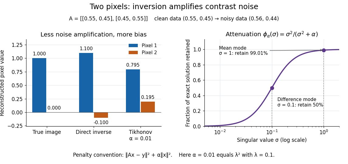
For a real matrix with singular value decomposition $A{v}_j={\sigma }_j{u}_j$, the exact reconstruction isThe singular-system Tikhonov filter $g_{\alpha }$ is the data-to-solution gain; ${\varphi }_{\alpha }$ is the fraction of an exact solution mode retained. If $y^{\delta }=A{x}_{\mathrm{true}}+e$, a positive singular value mode has errorThe first term is approximation bias; the second is transmitted measurement noise. Suppressing a weak mode suppresses its true signal too.

For the two-pixel matrix in the inverse problem example and $\alpha =0.01$ ($\lambda =0.1$), the mean and difference attenuation factors are $100/101$ and $1/2$. Since $y^{\delta }=q_{+}/\sqrt{2}+0.12q_{-}/\sqrt{2}$, the reconstruction isIts noise contribution is $(0.05,-0.05{)}^T$, half the direct inverse's, but its exact-data reconstruction is $(0.74505,0.24505{)}^T$. Consequently its total error Euclidean norm, about $0.28293$, exceeds the direct inverse's $0.14142$: this parameter sacrifices too much contrast. Taking $\alpha =0.001$ instead gives $(1.04496,-0.04595{)}^T$ and error about $0.06429$. Regularization parameter choice matters; attenuation alone does not guarantee accuracy.