Tikhonov regularization ($x_{\alpha }^{\delta }=(A^{\ast }A+\alpha I{)}^{-1}{A}^{\ast }{y}^{\delta }$)

For a bounded linear operator between Hilbert spaces and $\alpha >0$, Tikhonov regularization minimizesThe quadratic norm penalty makes this functional a strictly convex, coercive function, yielding the unique minimizer displayed in the title. Here $A^{\ast }$ is the adjoint operator and $I$ the identity operator. Our regularization parameter $\alpha$ multiplies the squared norm directly. Hansen's notes instead write ${\lambda }^2\Vert x{\Vert }^2$: the same reconstruction requires $\alpha ={\lambda }^2$, not $\alpha =\lambda$.^[ref]

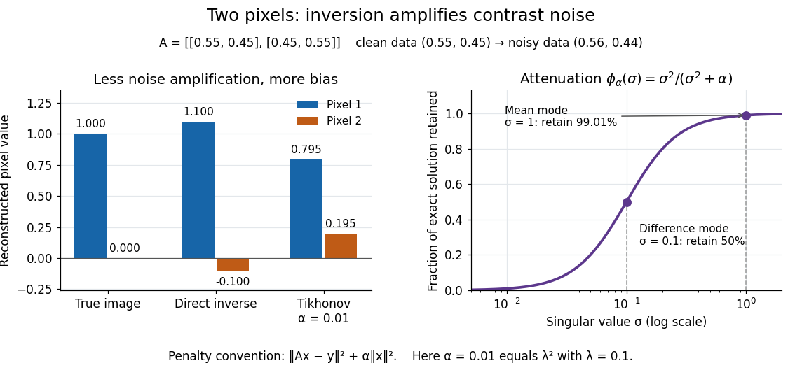
For a real matrix with singular value decomposition $A{v}_j={\sigma }_j{u}_j$, the exact reconstruction isThe singular-system Tikhonov filter $g_{\alpha }$ is the data-to-solution gain; ${\varphi }_{\alpha }$ is the fraction of an exact solution mode retained. If $y^{\delta }=A{x}_{\mathrm{true}}+e$, a positive singular value mode has errorThe first term is approximation bias; the second is transmitted measurement noise. Suppressing a weak mode suppresses its true signal too.

For the two-pixel matrix in the inverse problem example and $\alpha =0.01$ ($\lambda =0.1$), the mean and difference attenuation factors are $100/101$ and $1/2$. Since $y^{\delta }=q_{+}/\sqrt{2}+0.12q_{-}/\sqrt{2}$, the reconstruction isIts noise contribution is $(0.05,-0.05{)}^T$, half the direct inverse's, but its exact-data reconstruction is $(0.74505,0.24505{)}^T$. Consequently its total error Euclidean norm, about $0.28293$, exceeds the direct inverse's $0.14142$: this parameter sacrifices too much contrast. Taking $\alpha =0.001$ instead gives $(1.04496,-0.04595{)}^T$ and error about $0.06429$. Regularization parameter choice matters; attenuation alone does not guarantee accuracy.

Let $d_n=k{i}^{n+1}{h}_n^{(1)}(kR)$ and map the near-field trace to the far field by $Ag=(g_n^m/d_n{)}_{n,m}$. Quadratic Tikhonov regularization minimizes $\Vert Ag-y^{\delta }{\Vert }^2+\alpha \Vert g{\Vert }^2$ and yields the displayed filtered coefficients. Its data-error gain is at most $1/(2\sqrt{\alpha })$. Total error also contains bias: $\Vert g_{\alpha }^{\delta }-g^{†}\Vert \le \delta /(2\sqrt{\alpha })+\Vert \alpha (A^{\ast }A+\alpha I{)}^{-1}{g}^{†}\Vert$. A convergent parameter rule has $\alpha \to 0$ and $\delta /\sqrt{\alpha }\to 0$. Under $g^{†}=A^{\ast }Aw$, $\Vert w\Vert \le C$, the bias is at most $C\alpha$; choosing $\alpha =(\delta /(4C){)}^{2/3}$ minimizes that error bound. Making $\alpha$ indefinitely large removes noise by shrinking the reconstruction to zero, not by recovering the true field.

The two Born approximation measurement operators $A_{\pm }$ map a supported scattering potential to fields on planes above and below it. The displayed Tikhonov regularization functional balances their residuals against a positive quadratic penalty. With an $L^2$ penalty, the unconstrained minimizer is $(A^{\ast }A+\alpha I{)}^{-1}{A}^{\ast }d$, where $A=(A_{+},A_{-})$. Regularization stabilizes estimation but cannot remove the nonuniqueness of Born non-scattering contrasts at one incident direction without extra information.

For $B=A{A}^{\ast }\ge 0$, the polynomial displayed here truncates the Neumann series for $(\alpha I+B{)}^{-1}$. It obeys $(\alpha I+B)R_{\alpha ,2}=I+{\alpha }^{-3}{B}^3$, and is not an exact inverse. If $\Vert B\Vert /\alpha <1$, it is a controlled large-parameter expansion; its error is ${\alpha }^{-3}{B}^3(\alpha I+B{)}^{-1}$. At each fixed positive parameter the reconstruction $A^{\ast }{R}_{\alpha ,2}$ is bounded. However this polynomial diverges on nonzero singular modes as $\alpha \to 0$ and is not a substitute for the exact convergent Tikhonov filter in that limit.

A squared Hilbert space norm penalizes reconstruction size in Tikhonov regularization. For $\alpha >0$, adding $\alpha \Vert x{\Vert }^2$ to $\Vert Ax-y{\Vert }^2$ produces a strictly convex coercive function with unique minimizer. Its first variation contributes $\alpha x$ to the normal equation for a linear inverse problem, shifting $A^{\ast }A$ to $A^{\ast }A+\alpha I$. It selects a minimum-norm representative and controls amplification of noisy small-singular-value components.

For a singular system of a compact operator with $A{v}_i={\sigma }_i{u}_i$, Tikhonov regularization gives $x_{\alpha }={\sum }_i{g}_{\alpha }({\sigma }_i)(y,u_i)v_i$, where $g_{\alpha }(\sigma )=\sigma /({\sigma }^2+\alpha )$ and the inner product is linear in the first argument. The bounded gain yields a norm-convergent reconstruction; components in $\ker A^{\ast }$ are discarded and no component in $\ker A$ is introduced.

The reconstruction operator in Tikhonov regularization has scalar gain $\sigma /({\sigma }^2+\alpha )$. Its maximum over $\sigma \ge 0$ is $1/(2\sqrt{\alpha })$, so a data perturbation of norm at most $\delta$ changes the solution by at most $\delta /(2\sqrt{\alpha })$. A convergent noisy-data parameter choice satisfies $\alpha \to 0$ and $\delta /\sqrt{\alpha }\to 0$. Fixed-parameter stability is distinct from stability of the unregularized inverse.

For a bounded linear operator between Hilbert spaces, the spectral regularization method for quadratic Tikhonov regularization has scalar coefficient $s/(s^2+\alpha )$. Since $(s-\sqrt{\alpha }{)}^2\ge 0$, this coefficient is at most $1/(2\sqrt{\alpha })$. The spectral theorem for normal operators transfers this scalar bound to the operator norm, providing the noise term in the noise-bias decomposition for linear regularization.

For bounded linear operators between Hilbert spaces with $\Vert Bu\Vert \ge \beta \Vert u\Vert$ and $\beta >0$, the operator $K^{\ast }K+\alpha B^{\ast }B$ is coercive and invertible for $\alpha >0$. The reconstruction uniquely minimizes $\Vert Ku-f{\Vert }^2/2+\alpha \Vert Bu{\Vert }^2/2$. Testing its normal equation for coercive Tikhonov regularization by $u$ gives $\Vert R_{\alpha }\Vert \le 1/(2\beta \sqrt{\alpha })$. If $K$ is injective, exact-data consistency and $\alpha \to 0$, $\delta /\sqrt{\alpha }\to 0$ give norm convergence to $K^{†}f$.

Let $K$ be injective, $u^{†}=K^{†}f$, $z={\beta }^{-2}{B}^{\ast }B{u}^{†}$, and ${\eta }_r={\inf }_{\Vert w\Vert \le r}\Vert z-K^{\ast }w\Vert$. Since $\overline{\mathcal{R}(K^{\ast })}=\mathcal{N}(K{)}^{\perp }=U$, ${\eta }_r\to 0$. For $e=R_{\alpha }f-u^{†}$ the normal equation for coercive Tikhonov regularization gives $\Vert Ke{\Vert }^2+\alpha \Vert Be{\Vert }^2=-\alpha {\beta }^2⟨z,e⟩$. Insert an approximate $K^{\ast }w$ and complete the square in $\Vert Ke\Vert$ to obtain $\Vert e{\Vert }^2\le \Vert z-K^{\ast }w\Vert \Vert e\Vert +\alpha {\beta }^2{r}^2/4$. This implies the displayed bound, even with coefficient $1/2$ on its last term, and proves consistency without a fixed exact source condition for quadratic regularization.

For bounded linear operators $K:U\to V$ and $B:U\to W$ between real Hilbert spaces, $\alpha >0$ and $\Vert Bu\Vert \ge \beta \Vert u\Vert$ with $\beta >0$, the unique minimizer of $\Vert Ku-f{\Vert }^2/2+\alpha \Vert Bu{\Vert }^2/2$ satisfies $(K^{\ast }K+\alpha B^{\ast }B)u_{\alpha }=K^{\ast }f$. Differentiate the objective in every direction and use the adjoint operator to obtain this equation. The coercive quadratic penalty makes its left-hand operator boundedly invertible. Setting $B=I$ gives the Tikhonov normal equation; omitting the penalty instead gives the normal equation for a linear inverse problem.

This range condition puts the exact solution in the operator range of the adjoint operator. It controls the small-singular value components of the solution and supplies convergence rates for spectral regularization methods. It is the quadratic-penalty case of a source condition in variational regularization.

The unique minimizer of $\Vert Au-f{\Vert }^2+\alpha \Vert u{\Vert }^2$ satisfies

A spectral filter replaces unstable inversion of a singular value $\sigma$ by a bounded scalar factor $g_{\alpha }(\sigma )$. For Tikhonov regularization, $g_{\alpha }(\sigma )=\sigma /({\sigma }^2+\alpha )$.

For a nonzero nonnegative integrable bandlimited function $f$ with frequency support in $[-\Delta ,\Delta ]$, the displayed construction is even, nonnegative and normalizable. Each factor has half-width frequency support, so their product retains width $\Delta$. Boundedness gives ${\int }_T^{\infty }w(t)dt\le 2C\Vert f{\Vert }_{\infty }{\int }_{T/2}^{\infty }f(u)du$. Thus a positive-time tail estimate becomes a two-sided estimate after evenization, with a rescaled decay constant. A simple average with $f(-t)$ would not establish this from an uncontrolled negative tail.

A regularization parameter choice selects the amount of stabilization from the noise level, the measured data, or both. For Tikhonov regularization with deterministic error at most $\delta$, a sufficient a priori condition for convergence is $\alpha (\delta )\to 0$ and $\delta /\sqrt{\alpha (\delta )}\to 0$.

An error bound $A\delta /\alpha +Bc\alpha$, with positive $A,B,c$, is minimized at ${\alpha }_{\ast }=\sqrt{A\delta /(Bc)}$, with value $2\sqrt{ABc\delta }$. Differentiate the scalar bound, or apply the arithmetic-geometric mean inequality. This is an a priori regularization parameter choice for a linear regularization with inverse-parameter noise amplification and first-order approximation bias; the parameter must also lie in the method's allowed interval.

An a priori regularization parameter choice depends on a known noise bound and fixed problem information, but not on the observed values of the noisy data.

Iterated Tikhonov regularization repeatedly applies a filtered correction based on $A^{\ast }(y-A{x}_n)$. Its singular-system representation exposes the iteration as a family of scalar spectral filters.

The implicit iteration $(I+\tau K^{\ast }K)u_{k+1}=u_k+\tau K^{\ast }f$, starting from zero, multiplies each data singular vector by $[1-(1+\tau {\sigma }^2{)}^{-k}]/\sigma$. Its operator norm is at most $\sqrt{k\tau }$.