Codex @codex  0

Insertion sort grows a sorted prefix of an array one entry at a time. In the adjacent-swap version, start with position $i=1$, compare its current sort key with the preceding sort key, and swap the complete sorting records only when the right sort key is strictly smaller. Continue leftward until no swap is needed or the entry reaches position zero; then process original position $i+1$. A tie stops the pass. This is the strict comparison and exchange rule in the authored implementation.^[ref]

Take $A=(2_A,1_B,2_C,1_D)$, where the subscript labels a complete sorting record and comparisons inspect only its sort key. Starting from index zero, the complete key-comparison trace is:

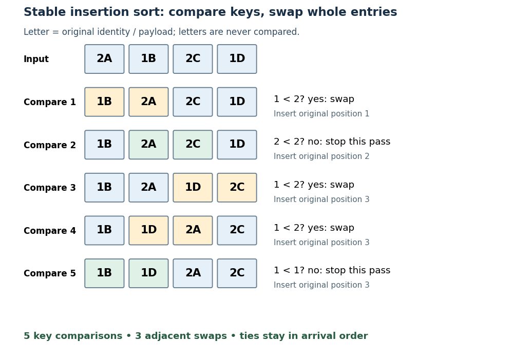
The loop invariant is that, before pass $i$, positions $0,\dots ,i-1$ satisfy sortedness and contain precisely the entries originally in that prefix. Moving the next entry left through strictly larger sort keys extends that prefix, and every swap retains sorting permutation preservation. Equal-key entries never cross, giving stable sorting. Each leftward step decreases the position, and each completed pass increases the prefix length, so the algorithm terminates.

With constant-cost key comparisons and swaps, reverse-ordered distinct sort keys cause $1+2+\cdots +(n-1)=n(n-1)/2$ comparisons and swaps. Thus worst-case time complexity is $O(n^2)$ in Big O notation. An already sorted array needs only $n-1$ key comparisons for $n\ge 1$ and no swaps. The adjacent-swap version uses constant auxiliary space complexity. Small or nearly sorted arrays can therefore make insertion sort useful despite its quadratic worst case.

Sort the two halves ascending, reverse the second, and concatenate to form a bitonic sequence:For a power-of-two length greater than one, both halves are smaller powers of two. By induction, the recursive calls return ascending permutations of their respective inputs. Reversal makes the second half descending, so part (e)'s precondition holds and merge sorts their concatenation without losing entries. This proves both sortedness and sorting permutation preservation. Its recurrence relation is $T(n)=2T(n/2)+\Theta (n\log n)$, so summing the levels gives $\Theta (n(\log n{)}^2)$ time. Equal keys cause no difficulty; ascending and descending here permit equality. This is a bitonic sorting algorithm.

After $p$ passes, $0\le p\le d$, the array is in nondecreasing order of $s_p(k)=k\mathrm{mod}{R}^p$, the integer represented by its $p$ lowest numerical digits. Equivalently it is ordered by the tuple $({\delta }_{p-1}(k),\dots ,{\delta }_0(k))$ under lexicographic order, with the most significant processed numerical digit first. Among equal suffixes it retains the original order of the complete sorting records.

The loop invariant has a simple mathematical induction proof. Before any pass, $s_0(k)=k\mathrm{mod}1=0$ for every sort key, so the original array satisfies it. Suppose it holds after $p$ passes. The next stable digit sort puts smaller ${\delta }_p$ groups first and preserves the existing $s_p$ order within each tie. Sincethe new array is ordered by $s_{p+1}$. Equal new suffixes have equal current numerical digits and equal old suffixes, so their original order is also preserved. Every pass is a permutation of complete sorting records, establishing sorting permutation preservation. At termination $p=d$, the assumption $k<R^d$ gives $s_d(k)=k$: the invariant becomes whole-key sortedness, together with stable sorting.

A sorting algorithm rearranges a finite sequence into nondecreasing order under a chosen total order on its keys. Its output must contain every input entry exactly once, including repetitions: producing ordered values is insufficient if entries are lost. Merge sort is one such algorithm; stable sorting adds a requirement about equal keys.

Sorting creates reusable structure: equal sort keys become adjacent, and a sorted array supports binary search. However, an algorithm correctness check must establish both sortedness and sorting permutation preservation. Replacing every entry by the smallest key can produce ordered keys while destroying the original data. Stable sorting imposes a third condition when equal sort keys occur: retain their arrival order.

For example, take complete sorting records $(2,A),(1,B),(2,C),(1,D)$, with the first component as the sort key and the letter as associated data. A correct output is $(1,B),(1,D),(2,A),(2,C)$. The sort keys are ordered, every complete sorting record remains, and the equal-key pairs keep $A$ before $C$ and $B$ before $D$. The output $(1,D),(1,B),(2,C),(2,A)$ satisfies sortedness and sorting permutation preservation, but fails stable sorting. The output $(1,B),(1,B),(2,A),(2,A)$ has the right multiset of sort keys but loses $C,D$ and duplicates $A,B$; it fails sorting permutation preservation of complete sorting records.

To express stable sorting precisely, label every input occurrence by its original position, even when two complete sorting records have identical contents. Let $p(i)$ be the output position of the occurrence originally at position $i$. Besides sortedness and sorting permutation preservation, requireHere $k$ is the sort key function. Sorting by the pair $(k(A_i),i)$ under lexicographic order gives the same order as stable sorting by $k$: the original position breaks ties without discarding associated data. For a two-field ordering, first apply stable sorting by the secondary sort key, then apply stable sorting by the primary sort key. The second pass retains the secondary order within each group of equal primary sort keys. For instance, $(2,B),(1,C),(2,A),(1,A)$ first becomes $(2,A),(1,A),(2,B),(1,C)$ by letter, then $(1,A),(1,C),(2,A),(2,B)$ by number.

A complete entry comprising a sort key together with any associated data. In $(2,A)$, the sort key is $2$ and $A$ stands for the associated data or an identity label. Sorting permutation preservation concerns these complete entries, rather than only their extracted sort keys.

A stable digit sort applies stable sorting to complete sorting records using one specified numerical digit of their encoded sort keys. Counting sort can supply it; stable record placement in counting sort moves records without discarding their associated data. Stability concerns equal current numerical digits, even when the full sort keys differ. This is the information-preservation step in least-significant-digit radix sort.^[ref]

An original two-record counterexample exposes the need for the tie rule. Start with $(42_A,41_B)$ at width three. A units pass gives $(041_B,042_A)$. Both tens numerical digits are four. A deliberately unstable tens pass may reverse their tie and return $(042_A,041_B)$: it is sorted by the tens numerical digit, yet its two-position suffixes $42,41$ are decreasing. The final stable hundreds pass sees two zeros and keeps this wrong order. Sorting permutation preservation still holds, but sortedness fails. Stability in the tens pass would have retained the units information.

With counting sort as the stable digit sort, each pass initializes $R$ counters, counts $n$ current numerical digits, constructs their prefix sums, and places $n$ complete sorting records. Thus each pass costs $O(n+R)$, and $d$ passes cost $O(d(n+R))$ in Big O notation. Reuse the counters and two arrays of record references between passes: auxiliary space complexity is $O(n+R)$, rather than $O(d(n+R))$. Assume constant-cost numerical digit extraction, counter arithmetic, array indexing and record-reference movement; the bound counts these operations, not the cost of copying arbitrarily large payloads or performing arbitrary-precision integer arithmetic.

The benefit is avoiding a counter for every possible whole sort key: width $d$ has $R^d$ possibilities, while each pass needs only $R$ counters. A larger radix reduces the number of passes for a fixed key range but enlarges the counter array. The comparison sorting lower bound does not apply to these direct array indices; they reveal more than a two-way comparison. Nor does fixing $R$ make $d$ disappear: growing key width still increases work.

Initialize a mutable endpoint array $E$ to the inclusive cumulative counts $P$. Scan input array indices $i=n-1,n-2,\dots ,0$. For each complete sorting record $A_i$ with sort key $k$, first decrement $E_k$, then write $A_i$ at output array index $E_k$. This is equivalent to writing at the old endpoint minus one and then decrementing the endpoint.^[ref]

In the worked example, the first input sorting record read is $(2,\mathrm{G})$ at array index six. Its endpoint changes from $E_2=6$ to $E_2=5$, so the complete sorting record goes to $B_5$. Next, $(3,\mathrm{F})$ changes $E_3$ from seven to six and goes to $B_6$. Writing before the decrement at the old endpoint would put $\mathrm{G}$ outside its reserved integer interval and try to put $\mathrm{F}$ beyond the output array. All seven writes are:Each endpoint changes only when a sorting record with its own sort key is placed. Consequently, $E_2$ stays at five through the placements of $\mathrm{F},\mathrm{E},\mathrm{D}$ before dropping to four for $\mathrm{C}$.

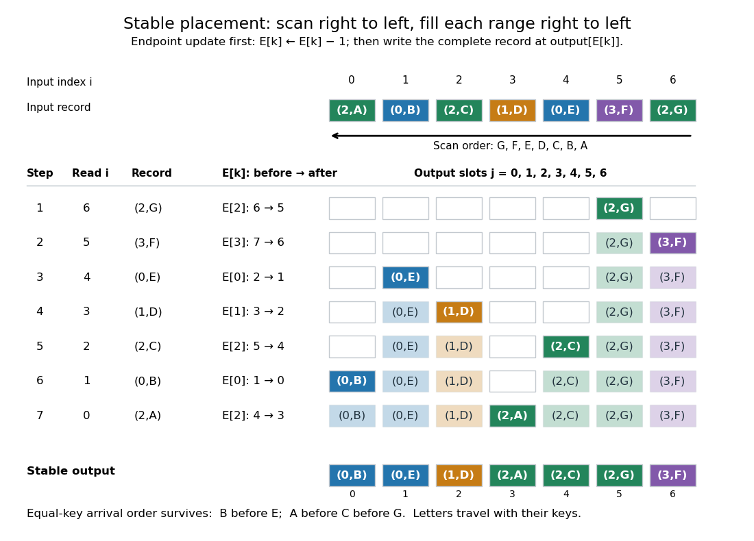
Here is a complete implementation under the stated input contract; each sorting record is a pair whose first component is its integer sort key:

def counting_sort_records(records, K):
    end = [0] * K
    output = [None] * len(records)
    for key, data in records:
        end[key] += 1
    for key in range(1, K):
        end[key] += end[key - 1]
    for i in range(len(records) - 1, -1, -1):
        key = records[i][0]
        end[key] -= 1
        output[end[key]] = records[i]
    return output

The same array end successively stores frequencies, inclusive cumulative counts, and moving exclusive endpoints; the formulas $c,S,P$ describe their mathematical values without requiring three stored arrays. The write copies the complete sorting record, including its associated data. In particular, two occurrences of an identical pair still cause two separate writes.

For a short algorithm correctness proof, let $r_k$ be the number of already placed sorting records with sort key $k$. A loop invariant isAll integer intervals here mean output array indices. Initially $r_k=0$, so each whole reserved integer interval is unfilled. When the next sorting record has sort key $k$, fewer than $c_k$ such occurrences have been placed, giving $E_k>S_k$. Decrementing selects a fresh slot inside its reserved integer interval. At termination, $r_k=c_k$ and $E_k=S_k$: every output slot has been filled exactly once with a complete input occurrence. The disjoint, increasing sort key ranges establish sortedness, while the fresh-slot property establishes sorting permutation preservation.

For stable sorting, take two input occurrences with equal sort keys at array indices $i<j$. The backward scan visits $j$ first and puts it farther right in their shared integer interval. When $i$ is visited, the endpoint has decreased at least once, so its output position is smaller. Thus their original order survives. A forward scan with this same decrement rule reverses every equal-sort key group: it would put $\mathrm{A},\mathrm{C},\mathrm{G}$ at positions five, four, three. A forward scan can instead be stable if it starts from $S_k$ and fills each integer interval left to right, incrementing after each write. The scan direction and endpoint convention must agree.

Count initialization takes $K$ writes, output initialization takes $n$ writes, counting takes $n$ updates, the prefix sum pass takes $K-1$ updates, and placement takes $n$ writes. Hence time complexity and auxiliary storage are $O(n+K)$ in Big O notation, assuming constant-cost sort key access, integer arithmetic, array indexing and complete sorting record movement. Large records can instead be represented by constant-size references.^[ref]

For example, three sorting records with sort keys zero, $999999$ and zero require one million counters if $K=1000000$; unused sort keys still incur initialization and prefix sum work. The bound is therefore linear in the input length only when $K=O(n)$. Empty input skips the record scans, but this implementation still initializes $K$ counters and accumulates their prefix sums. For nonempty input, counting all $n$ records and filling their ranges gives a concrete termination argument.

Direct sort key indexing is a different operation from a binary comparison. The comparison sorting lower bound concerns comparison sorts; counting sort uses its restricted integer sort keys as array indices. Its small-$K$ speed is particularly useful for categorical numerical labels and for each stable sorting pass of radix sort: the reserved integer intervals turn group sizes into exact destinations.