For an equally populated ideal pair of angular momentum eigenstates, the magnetic moment component takes two values, , and the displacements at fixed velocity are . Compare a specified classical alternative: every chemical atom carries a permanent magnetic moment of fixed magnitude , with independently isotropic initial orientations and no dissipative alignment. If , the sphere's area element is , so has a uniform distribution on . With precession preserving this component in the ideal geometry, the displacement fills the interval continuously. A pair of bands therefore tests allowed components rather than merely proving that silver is magnetic. Other classical preparation assumptions would be different models and must be stated.
To include finite instrumental width, choose a normalized Gaussian distributionwith standard deviation , representing a combined field-off spatial width. At fixed velocity the model probability density functions areEach has unit integral and zero mean; the different shapes, rather than a different average displacement, distinguish them. The discrete model has variance , whereas the classical model has variance . Their common mean also explains why the raw average landing position is insufficient to identify the internal quantum state.
Now choose a uniform distribution of forward velocities from to , explicitly as an example rather than the oven's actual distribution. Average either conditional probability density function over that interval. The positive-channel displacement ranges from to , since slower chemical atoms spend longer accelerating and drifting. The two components broaden into bands even though their internal magnetic moment values remain discrete. The corresponding classical profile continues to populate the center. The displayed strip darkness is proportional to predicted deposited number density, with equal total arrivals; it is not a photograph or a calibrated optical response of a developed film.
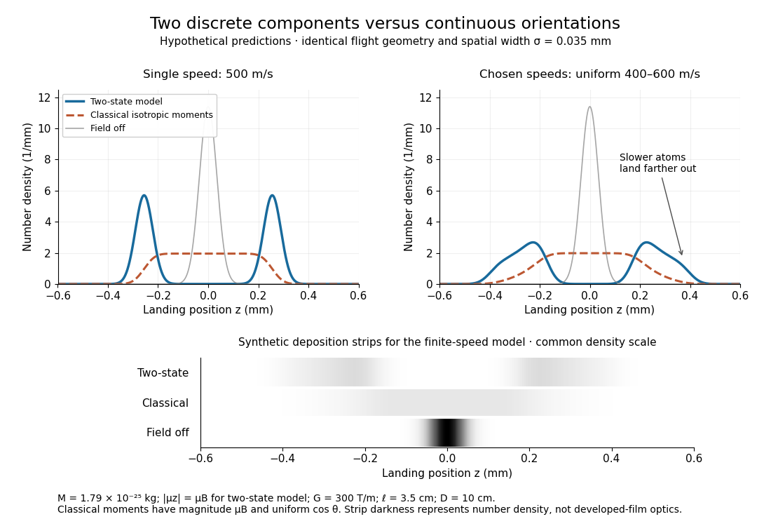
Discrete magnetic components and continuous classical deflections
. Original model predictions with the chosen flight parameters, comparing one forward speed with a finite speed interval. Both alternatives include the same Gaussian spatial width. Synthetic deposition strips use a common density scale; none of the curves or strips is measured data. Details.
Increasing the spatial width until it is comparable with can hide the two maxima. At fixed velocity, differentiating the two-state probability density function twice gives : the central minimum becomes a central maximum when . Conversely, a broad distribution of velocities need not create a new internal component: it spreads each existing component through the dependence. Further instrumental limits include collisions, aperture clipping of strongly deflected trajectories, asymmetric pole geometry, and nonlinear film development. Field-off widths and a mapped magnetic field gradient are needed to separate such effects. For a modern counting experiment, channel calibration and efficiency corrections belong to Stern-Gerlach expectation estimation; spatial separation alone does not supply those statistics.
Articles by others on the same topic
There are currently no matching articles.