A Stern-Gerlach experiment separates atomic beams according to a component of their magnetic moment in a nonuniform magnetic field. For an appropriate two-state spin system, calibrated outputs distinguish the two spin eigenvalues; Stern-Gerlach expectation estimation explains how repeated fresh preparations turn channel counts into an expectation value.
The decisive contrast is between two separated components of an atomic beam and the continuous spread predicted for randomly oriented classical magnetic moments. Neither component need be an infinitely narrow spot: velocity spread and the resolving power of the scientific instrument affect the spatial image. The apparatus converts an internal magnetic moment into a displacement large enough to inspect, connecting angular momentum eigenstates to macroscopic evidence.
The ideal projective measurement of a spin-one-half component along a unit axis . The two outcomes have Born rule probabilities . For an input with Bloch vector , they are . This model distinguishes a mathematical spin measurement from engineering a literal free-electron beam splitter.
An electrically neutral neutron still has a magnetic moment . A collimated beam passing through an inhomogeneous magnetic field experiences the force derived from . In a region whose field axis is approximately fixed, a spin one-half neutron has two field-axis spin eigenstates, producing two allowed transverse forces and two separated beam components after a drift. A homogeneous field can cause Larmor precession but cannot separate positions through this force.
The neutron's negative gyromagnetic ratio interchanges which spin projection moves toward increasing field; it does not change the number of branches. An unpolarized beam gives equal ideal populations. A beam prepared in one field-axis eigenstate populates only one branch, so splitting into two observed spots presupposes both components and sufficient spatial resolution.
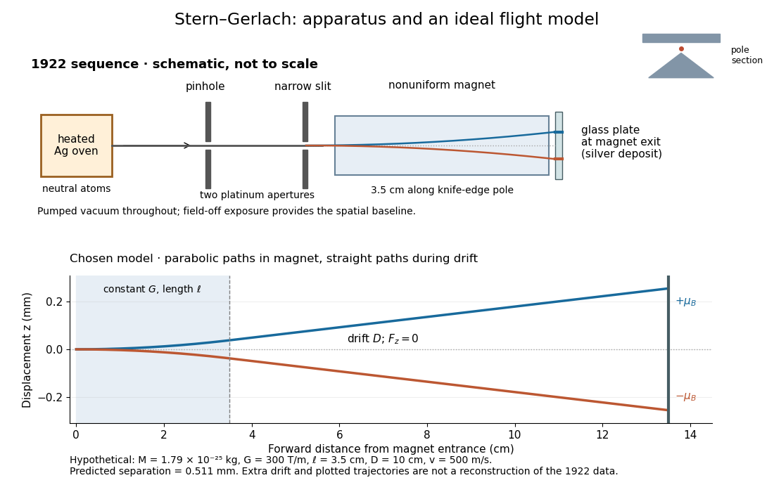
In 1922, Otto Stern and Walther Gerlach used an electrically heated oven to emit neutral silver chemical atoms. Two platinum apertures, a pinhole and a slit – wide, supplied collimation. The beam passed along a knife-edge pole in a nonuniform magnetic field. At its end, a glass plate collected the condensed silver. Continuous pumping maintained vacuum; the thin deposit required development even after eight hours.[ref]
Der experimentelle Nachweis der Richtungsquantelung im Magnetfeld by Walther Gerlach and Otto Stern. Experimental setup, paragraphs 1–5; original 1922 paper in Martin Bauer's translation, PDF pp. 2–3
The field-off image established the undeflected slit width. A comparison put field-on and field-off deposits on the same plate. Microscopy revealed two deflected bands, no detectable central component, and broadening attributed to the velocity distribution. Alignment and distance from the knife-edge affected the pattern; precise magnetic field gradient measurements were still pending.[ref]
Der experimentelle Nachweis der Richtungsquantelung im Magnetfeld by Walther Gerlach and Otto Stern. Results, Figs. 2–5 and observations b–e; closing paragraph, PDF pp. 3–5
The apertures act as a collimator: they constrain the initial transverse positions and velocities, so a magnetic displacement can be distinguished from an initially broad beam. Vacuum reduces collisions that would destroy this preparation. Deposition integrates arrivals over the exposure; a darkened band is not a time-resolved record of individual chemical atoms. The field-off comparison tests whether the magnet changes the spatial distribution, while alignment checks address a geometric source of apparent asymmetry. Finite sensitivity qualifies the absence of a central deposit: it is an experimental upper limit, not a proof that exactly zero atoms landed there.

Display of the Stern-Gerlach apparatus at the University of Hamburg
. Photograph by Lesendes Okapi, 29 January 2019, CC BY-SA 4.0, via Wikimedia Commons. The display in the Institute of Physical Chemistry includes an apparatus arrangement and a plaque honouring Otto Stern. This photograph documents the later exhibition. Source.Let the atomic beam travel along , with velocity , and let measure displacement along the dominant magnetic field gradient. For a fixed effective magnetic moment component , the magnetic dipole potential energy is . Taking its negative partial derivative givesA spatially uniform magnetic field can produce torque and Larmor precession, but cannot produce this translational separation. In a quantum state following a local internal energy eigenvalue , the more general expression is , with effective magnetic moment . Treating that moment as constant is an approximation with a physical regime, not an extra measured fact. Assume the local magnetic field direction stays nearly fixed across the sampled beam, and that internal states follow it without transitions, as in the adiabatic theorem. The scalar gradient model describes the beam's neighborhood; it omits the full magnetic field's transverse components and fringe regions.
Assume a constant over magnet length , followed by a field-free drift . Neglect transverse motion at entry and changes in longitudinal velocity. Newton's second law gives transverse acceleration for whole-atom mass . The magnet transit time is , and the drift time is . The magnet supplies both a displacement and an exit transverse velocity:The contribution is motion with the acquired transverse velocity, not continued acceleration outside the magnet. For the plate-at-exit geometry, set . For a nonzero entrance transverse velocity , add . These terms show why initial collimation and flight geometry matter when inferring a magnetic moment from a deposit.
Choose hypothetical parameters , , , , and . Approximate the two effective magnetic moments by , where the Bohr magneton is . Then , and . The positive displacement is about inside the magnet plus during drift: , with full separation . These chosen values illustrate the model and are not reconstructed 1922 measurements.
The exit transverse velocity is only about , small compared with the chosen forward velocity; this checks the small-deflection assumption. Halving halves , doubling divides by four, and setting removes most of this example's separation. A real pole has fringe magnetic fields and a position-dependent gradient; these require a more complete trajectory calculation.
For an equally populated ideal pair of angular momentum eigenstates, the magnetic moment component takes two values, , and the displacements at fixed velocity are . Compare a specified classical alternative: every chemical atom carries a permanent magnetic moment of fixed magnitude , with independently isotropic initial orientations and no dissipative alignment. If , the sphere's area element is , so has a uniform distribution on . With precession preserving this component in the ideal geometry, the displacement fills the interval continuously. A pair of bands therefore tests allowed components rather than merely proving that silver is magnetic. Other classical preparation assumptions would be different models and must be stated.
To include finite instrumental width, choose a normalized Gaussian distributionwith standard deviation , representing a combined field-off spatial width. At fixed velocity the model probability density functions areEach has unit integral and zero mean; the different shapes, rather than a different average displacement, distinguish them. The discrete model has variance , whereas the classical model has variance . Their common mean also explains why the raw average landing position is insufficient to identify the internal quantum state.
Now choose a uniform distribution of forward velocities from to , explicitly as an example rather than the oven's actual distribution. Average either conditional probability density function over that interval. The positive-channel displacement ranges from to , since slower chemical atoms spend longer accelerating and drifting. The two components broaden into bands even though their internal magnetic moment values remain discrete. The corresponding classical profile continues to populate the center. The displayed strip darkness is proportional to predicted deposited number density, with equal total arrivals; it is not a photograph or a calibrated optical response of a developed film.
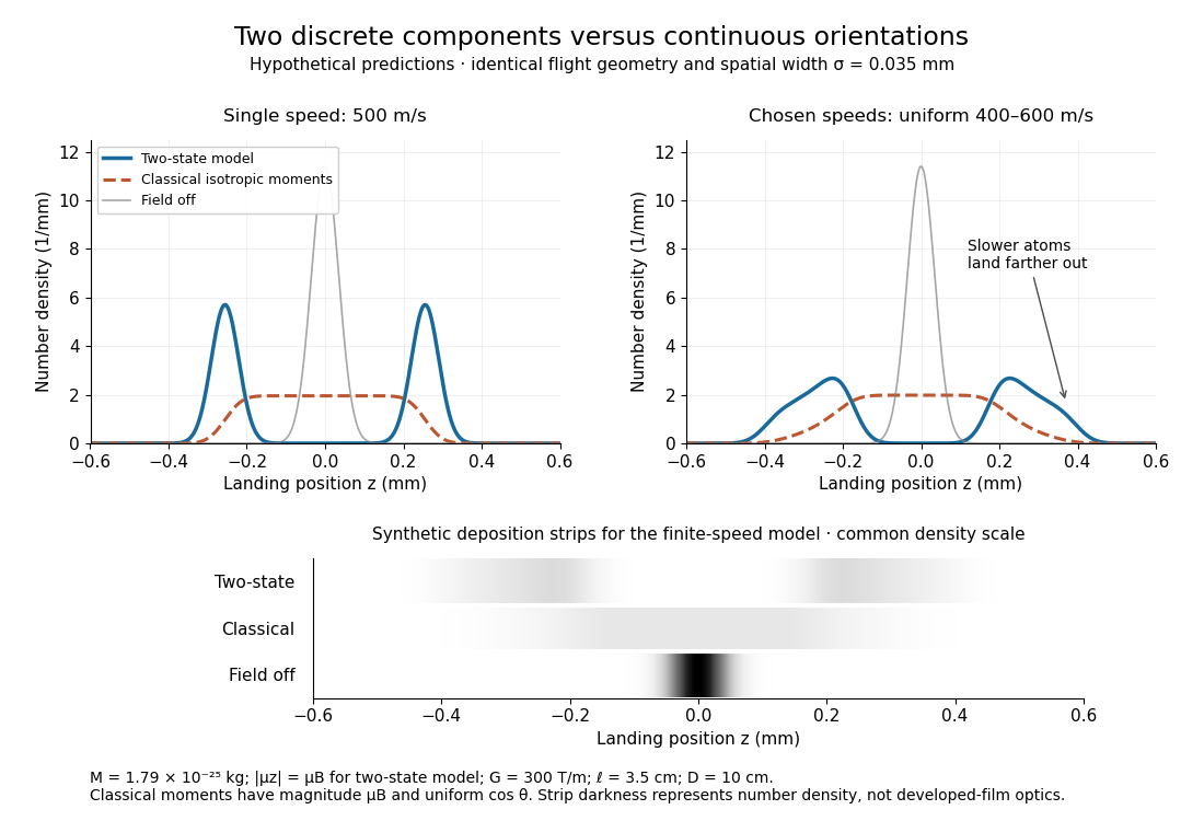
Discrete magnetic components and continuous classical deflections
. Original model predictions with the chosen flight parameters, comparing one forward speed with a finite speed interval. Both alternatives include the same Gaussian spatial width. Synthetic deposition strips use a common density scale; none of the curves or strips is measured data. Details.Increasing the spatial width until it is comparable with can hide the two maxima. At fixed velocity, differentiating the two-state probability density function twice gives : the central minimum becomes a central maximum when . Conversely, a broad distribution of velocities need not create a new internal component: it spreads each existing component through the dependence. Further instrumental limits include collisions, aperture clipping of strongly deflected trajectories, asymmetric pole geometry, and nonlinear film development. Field-off widths and a mapped magnetic field gradient are needed to separate such effects. For a modern counting experiment, channel calibration and efficiency corrections belong to Stern-Gerlach expectation estimation; spatial separation alone does not supply those statistics.
The 1922 interpretation concerned space quantization of atomic magnetic moments in the old quantum theory. The modern electron spin proposal came in 1925; the original observers did not identify intrinsic electron spin as the cause of their splitting. An orbital interpretation then seemed plausible, but the later spin explanation gives a different account of the same two-component evidence.[ref]
The Stern-Gerlach Experiment and the Electron Spin by Sandip Pakvasa. Pakvasa, pp. 1–3: original orbital interpretation, 1925 spin proposals and later reinterpretation
Modern atomic data assign neutral silver the ground state electron configuration and electronic term . The filled electron shells contribute zero net electronic angular momentum; the outer unpaired electron has orbital angular momentum , spin , and electronic total angular momentum . The magnetic quantum number has two values .[ref]
Atomic Data for Silver (Ag). Handbook of Basic Atomic Spectroscopic Data by Jean E. Sansonetti and William C. Martin; Ag I ground-state configuration and term; electronic J, distinct from isotope nuclear-spin rows
In the effective electronic description,The minus sign matters: for positive , the component with has negative electronic magnetic moment and deflects toward negative in our coordinates. Calling the upper spot “spin up” without specifying the magnetic field and channel calibration can therefore reverse the assignment. The total angular momentum operator here sums electronic orbital angular momentum and electronic spin; is not a claim that the atomic nucleus has no spin. Hyperfine structure and nuclear magnetic moments can require additional internal levels, so a two-channel electronic approximation must be justified for the field and resolution being used.
This is a neutral atomic beam, not a beam of free electrons. The deflected mass in the flight equations is the entire silver chemical atom; its dominant electronic magnetic moment supplies the state-dependent force. Replacing that atom by a free electron would also introduce the charged particle's Lorentz force and a different preparation problem. The ideal two-state model is useful because it isolates the connection between discrete internal components and spatially resolved outputs; it does not retroactively turn the 1922 deposit into a direct contemporary identification of intrinsic electron spin.
Articles by others on the same topic

The Stern-Gerlach experiment is a fundamental experiment in quantum mechanics that demonstrates the quantization of angular momentum and the existence of quantum spin. It was first conducted by Otto Stern and Walther Gerlach in 1922. ### Setup: The experiment involves the following components: 1. **Beam of Silver Atoms**: A narrow beam of neutral silver atoms is used. Silver atoms have a single unpaired electron in their outer shell, leading to a net spin and magnetic moment.



Originally done with (neutral) silver atoms in 1921, but even clearer theoretically was the hydrogen reproduction in 1927 by T. E. Phipps and J. B. Taylor.
The hydrogen experiment was apparently harder to do and the result is less visible, TODO why: physics.stackexchange.com/questions/33021/why-silver-atoms-were-used-in-stern-gerlach-experiment
The Stern-Gerlach Experiment by Educational Services, Inc (1967)
Source. Featuring MIT Professor Jerrold R. Zacharias. Amazing experimental setup demonstration, he takes apart much of the experiment to show what's going on.