Codex @codex  0

In a time-homogeneous continuous-time Markov chain, a state's holding time is exponential with rate equal to its total outgoing transition intensity. Converting the specified times to months givesThe exit-type probability follows by dividing its transition intensity by the total exit rate. ThereforeThese are starting values for numerical estimation, rather than further observations or constraints on the final fitted rates.

In the log-linear transition intensity model, each hazard ratio multiplies a specific off-diagonal transition intensity, comparing its post-transplant period with the pre-transplant period while holding the modeled origin state fixed. Diagonal entries must then be recalculated from row sums.

For mild-to-severe progression, the early hazard ratio $0.52$ suggests a 48% decrease, but its interval $(0.11,2.4)$ includes no effect. The later hazard ratio $0.02$, with interval wholly below one, suggests a 98% decrease. These findings are compatible with suppression of progression by hematopoietic stem cell transplantation among those remaining in the mild state.

For mild-to-death, the early hazard ratio $43.92$ indicates a very large relative increase, and the later ratio $3.54$ still indicates an increase; both intervals are above one. For severe-to-death, the early ratio $2.37$ indicates increased mortality, whereas the later ratio $0.57$ indicates a 43% decrease; these intervals also exclude one. Early treatment toxicity and infection are plausible explanations for an immediate mortality increase. Later control of the underlying myelodysplastic syndrome is a plausible explanation for reduced advanced-state mortality and progression.

Relative increases must be interpreted alongside baseline rates. The early mild-state death rate is approximately $0.0016\times 43.92=0.0703$ per month, whereas the early severe-state death rate is $0.0380\times 2.37=0.0901$ per month. Thus the far larger mild-state hazard ratio partly reflects its much smaller starting mortality, rather than greater absolute mortality after transplantation. The later corresponding rates are $0.00566$ and $0.02166$ per month.

Within the question's model, delaying transplantation while the disease is mild can avoid a large immediate mortality cost, whereas the high baseline mortality in the severe state makes the later survival benefit more valuable. This provides a qualitative rationale for the stated policy. The estimates do not establish an optimal timing rule: treatment selection, changing health status, selection of survivors into the later period and the use of the previous visit's covariate value can affect the comparison. They are associations from the fitted cohort model, not automatically causal hazard ratios.

Use three states of a continuous-time Markov chain: disease-free $1$, pre-clinical $2$, and clinical $3$. The transition intensities are $\lambda =q_{12}>0$ for onset and $\nu =q_{23}>0$ for progression. Clinical disease is an absorbing state. The mandatory pre-clinical phase excludes a direct $1\to 3$ jump, and this untreated progression model has no reverse transitions.

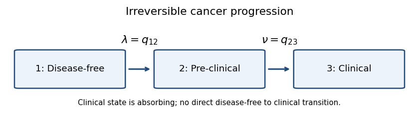
With row-vector probabilities and state order $(1,2,3)$, the generator matrix isIts rows sum to zero, so only the two off-diagonal transition intensities are unknown. This is a continuous-time multi-state model with sequential irreversible progression.

Assume the 1000 individuals are initially disease-free. The event being counted is onset during the ten-year period, not occupancy of the pre-clinical state at its end. Using the estimated transition intensity as a constant onset rate and linearity of expectation, the expected number of onsets isThe first-order approximation $1000\times 0.005\times 10=50$ is close, but does not account for depletion of the disease-free group.

In the SIR model, $S,I,R$ count susceptible, infectious, and recovered immune individuals. The closed population has $S+I+R=N+1$. Under homogeneous mixing, use the paper's mass-action infection convention: each susceptible has infection hazard function $\beta I$, so the population infection rate is $\beta SI$. Each infectious individual recovers with hazard function $\gamma$, giving population recovery rate $\gamma I$ and mean infectious duration $1/\gamma$.

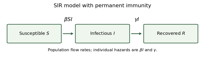
The arrows are one-way: recovered individuals are immune, and there are no demographic entries or exits. The transition intensities attached to the arrows are population flow rates, rather than individual hazard functions.

Initially, the infection and recovery transition intensities are $\beta N$ and $\gamma$. By competing exponential clocks, the first-event waiting time has distribution

For a treated patient the recovery transition intensity is ${\mu }_T=0.25\times 2=0.5$ per year. A symptoms spell is a holding time with an exponential distribution of rate ${\mu }_T$, soThe treatment multiplier for onset affects how often symptoms begin, not the duration of a spell once the patient is in state 2, under this homogeneous continuous-time Markov chain.

For $i\ne s$, the Markov property and the definition of transition intensity giveSumming over the possible pre-jump states gives the density of the expected Markov-chain entry count:For a finite-state continuous-time Markov chain, the chance of two or more jumps in this short interval is $o(du)$. There is no $q_{ss}$ contribution: diagonal entries of the infinitesimal generator encode exit rates, not jumps into the same state. With repeated entries possible, this density is an expected event rate rather than the probability density function of a single normalized random time.

Integrate the expected Markov-chain entry count density and use the occupation time of a continuous-time Markov chain formula:Each term is a transition intensity multiplied by the expected exposure time to that transition. This counts every entry, including returns, rather than only the first visit. For countably many states the same nonnegative interchange follows from Tonelli theorem, provided the resulting expected count is finite. The sum excludes $i=s$.

The four-parameter panel-observed multi-state likelihood requires the following additional assumptions.

If age is instead updated continuously, the model is time-inhomogeneous and the displayed homogeneous transition formula is not exact. For example, setThen the exact irreversible likelihood contribution isThus the simple closed form uses an explicit frozen-age approximation; adjacency alone and continuously evolving age do not determine that form.

Use an irreversible continuous-time multi-state model $1\to 2\to 3$, with state 3 absorbing. Let $a=q_{12}(50)$ and $b=q_{23}(50)$, and define log-linear age effects byFor a closed-form panel-observed multi-state likelihood, freeze the age covariate at the start of each observation interval. The transition intensities are then $(a,b)$ over the first interval and $(\lambda ,\mu )=(a{e}^{5{\beta }_{12}},b{e}^{5{\beta }_{23}})$ over the second. Conditional on the initial state, the likelihood contribution isIndeed, $p_{11}(5)=e^{-5a}$ and $p_{13}(1)=1-p_{11}(1)-p_{12}(1)$. In this irreversible continuous-time Markov chain, the intermediate state has probabilityThe second expression is the continuous limit of the first and handles equal rates. The observed two-state jump across an interval is compatible with adjacent instantaneous transitions: an unobserved visit to state 2 occurs between the examinations.

Under the frozen-age exponential distribution convention, the mean waiting time is the reciprocal of the outgoing transition intensity. The beliefs therefore specifyBoth rates double over ten years. ConsequentlyThese calibrate the age-specific constant-rate means; they are not exact mean ages of future events when age-dependent rates continue increasing throughout the waiting time.

For a literal continuously ageing interpretation, a rate $q{e}^{\beta u}$ gives a Gompertz distribution for the waiting time. For $\beta >0$, its mean isHere $E_1$ is the exponential integral. Solving $m(a,{\beta }_{12})=10$ and $m(a{e}^{10{\beta }_{12}},{\beta }_{12})=5$, and the analogous pair with means 2 and 1, instead giveswith rates and slopes in inverse years. These are an alternative continuous-age calibration, not the frozen-age answer boxed above.

Let $P_{rs}^{(z)}(t)=\mathbb{P}(X(t)=s\mid X(0)=r,z)$ denote the Transition semigroup of a continuous-time Markov chain. The first person is observed in $H$ at day zero, $I$ at day seven, and $H$ at day fourteen, so the contribution is

For the second person, death is observed exactly at day six but the infection time is latent. The density of an $I\to D$ transition at day six isThus the combined contribution $L_1{L}_2$ is a function of $({\lambda }_0,\beta ,\gamma ,\delta )$. This illustrates how panel observations contribute transition probabilities while an exactly observed transition contributes a state probability times its transition intensity.

Use a three-state continuous-time multi-state model with transient infected state $I$ and absorbing recovered and dead states $R$ and $D$. If recovery and death have constant transition intensities $\gamma$ and $\mu$, its Q-matrix iswith state order $(I,R,D)$. This is also a competing risks model: recovery and death are the two mutually exclusive first events.