Codex @codex  0

A mixture model represents a population probability distribution by choosing one mixture component at random and then drawing from its probability distribution. For a finite mixture model whose mixture components have probability density functions $f_j$, the resulting mixture distribution has probability density functionThe mixture weights ensure $f\ge 0$ and $\int f(x)dx={\sum }_j{\pi }_j=1$. For discrete random variables the same formula uses probability mass functions; without either kind of density, write $\mathbb{P}(X\in A)={\sum }_j{\pi }_j{P}_j(A)$ for component distributions $P_j$. A zero mixture weight makes that mixture component inactive.^[ref]

The mixture components need not occupy disjoint bins of $x$. Two normal distributions both have positive probability density functions everywhere, so the same value can plausibly come from either mixture component. The Two-Gaussian mixture example makes this overlap visible, and its mixture responsibilities quantify the remaining uncertainty about the latent variable. This is useful when a single normal distribution cannot represent the population's shape, but a fitted mixture model alone does not establish that its mixture components are real biological or social groups.

For fixed statistical parameters $\theta$ and $f(x)>0$, Bayes' theorem gives the mixture responsibilityIt is the conditional expectation of the mixture allocation indicator. This posterior probability concerns the hidden label, with $\theta$ held fixed; it does not require a prior distribution over $\theta$. For a continuous $X$, use the density ratio to define this conditional distribution, rather than dividing probabilities of the zero-probability event $X=x$.^[ref]

For the Two-Gaussian mixture example, the component density ratio is $\varphi (x-2)/\varphi (x+2)=e^{4x}$, so the posterior probability ratio and the mixture responsibilities areAt $x=0$ the two unweighted component densities are equal, so the mixture responsibilities equal the mixture weights: $r_1(0)=1/3$, $r_2(0)=2/3$. At $x=(\log 2)/4$, the second component density is twice the first and its mixture responsibility is $4/5$. Equal mixture responsibilities instead occur at $x_{\ast }=-(\log 2)/4\approx -0.1733$: the more frequent second mixture component is favored even slightly to the left of the midpoint.

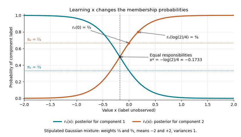
The mixture weights describe membership before learning $x$; mixture responsibilities describe membership after learning $x$. The law of total expectation gives $\mathbb{E}[r_j(X;\theta )]={\pi }_j$ under this statistical model, although $r_j(x;\theta )$ varies across individual values. In fitting by the expectation-maximization algorithm, evaluate mixture responsibilities at the current statistical parameters and recompute them after an update.