A latent variable is an unobserved random quantity introduced to describe dependence, hidden structure, or an indirect data-generating mechanism in a statistical model.
Persistent unmeasured differences between individuals can generate outcome dependence after adjusting for observed covariates. A random intercept is one representation. Conditional independence given that latent variable need not persist after it is integrated out; apparent history dependence can therefore occur without true state dependence.
Factor analysis writes an observation as , where the low-dimensional latent variable describes shared variation. In the isotropic Gaussian model and independently, the observation has covariance .
A latent factor is an unobserved coordinate introduced to explain shared variation among measurements. In an orthogonal factor model, latent factors have variance one and are mutually uncorrelated, with coefficients specified by the factor loadings. They differ from a regression factor, which is a categorical predictor. A fitted covariance alone generally leaves the latent factor orientation undetermined; factor rotation gives equivalent representations.
The latent factor vector has mean zero and covariance , the specific errors have mean zero and diagonal covariance , and the two are uncorrelated. Thus the off-diagonal covariance is explained by shared factors. Normality additionally gives a likelihood model, but the covariance identity needs only these second-moment assumptions. Positive diagonal entries of describe variation not explained by the factors. Unlike principal component analysis, the model separates shared and specific variation rather than only maximizing total projected variance.
An orthogonal rotation of factors leaves unchanged and hence preserves the model covariance. It proves rotational nonidentifiability of the unrestrained factor loadings. Choose an orientation for interpretability, for example varimax rotation, or impose identifying restrictions in a confirmatory model. An oblique transformation permits correlated factors: if becomes , their covariance becomes , preserving the same shared covariance.
An orthogonal factor rotation maximizing, over factor axes, the variance across variables of their squared loadings. It seeks an interpretable pattern with some large and many small loadings on each factor without changing the covariance fit.
The communality is the variance of the shared-factor contribution to variable . In an orthogonal factor model, , where is its specific variance. For standardized variables, . It measures variance shared through the modeled factors, not variance in a chosen principal component.
A factor loading is the coefficient of latent factor in observed variable . In the orthogonal factor model, . If has variance one, this is also its correlation with the variance-one factor. Its sign and size depend on the factor-coordinate convention; factor rotation preserves the implied covariance while changing individual loadings.
In factor analysis with one factor and fixed noise variance , let be the current loading vector, , and . The expectation-maximization algorithm update isThe conditional factor means are and their variances are ; maximizing the expected complete-data log-likelihood gives the formula.
A random effect is a latent variable used to describe variation between observational units or dependence among related observations. Its distribution supplements the fixed effects used in statistical modelling. Independent random effects produce extra variability; correlated random effects can produce serial dependence.
Let , with . The lognormal distribution of the random mean gives marginal mean . The law of total variance gives , strictly larger than when . Thus independent observation-level random effects produce overdispersion even though the conditional Poisson distributions have variance equal to their means.
Random effects are crossed when an observation can belong to levels of two grouping factors without one grouping factor being nested within the other. Independent location intercepts and incubator slopes, for example, contribute separate terms to the observation covariance matrix.
A random slope multiplies a predictor by a group-specific latent coefficient. With , a contribution induces covariance for two observations in group . A random slope does not necessarily include a random intercept.
When a person's latent slope has normal distribution , its th quantile is . Multiply by an elapsed time to obtain the corresponding latent change quantile. This describes population variation between people; it is distinct from a confidence interval for the mean slope and from a prediction interval that includes measurement error.
The Gaussian model with and independent has marginal law . Its group coefficients are integrated out of the marginal likelihood function. The special random-slope model uses predictor values in the grouping columns of .
The expectation-maximization algorithm fits a latent-variable model by alternating a conditional expectation over the latent variables with a maximization over the statistical parameters. Its target is the observed-data likelihood function, although its updates use the simpler complete-data log-likelihood.[ref]
Maximum Likelihood from Incomplete Data via the EM Algorithm by Arthur Pentland Dempster and others. Section 2, printed p. 6, equation (2.17) and the general E-step/M-step definition
Write for the observations, for the latent variables, and for their joint probability density function or probability mass function. The observed-data log-likelihood iswhere the integral becomes a sum for discrete . Directly maximizing a logarithm of this sum can be awkward. The E-step instead computes a conditional distribution at the current statistical parameters ; the M-step uses it to construct a new fit. The attractive idea is to retain uncertainty about the hidden labels while recovering simple weighted means and other complete-data updates. The Known-variance Gaussian mixture EM example shows the mechanism without estimating a variance or mixture weight.
Arthur Pentland Dempster, Nan M. Laird, and Donald B. Rubin gave the general framework its name in their 1977 paper, which also discusses earlier special-case algorithms.[ref]
Maximum Likelihood from Incomplete Data via the EM Algorithm by Arthur Pentland Dempster and others. Section 1, printed pp. 1 and 3: naming of the two steps and earlier special cases
Hold the old statistical parameters fixed when taking the conditional expectation, while keeping the candidate statistical parameters variable:For independent observations in a finite mixture model, is a hidden component label. Bayes' theorem gives its mixture responsibilities:These posterior probabilities are the conditional expectations of the mixture allocation indicators; they turn hidden counts into fractional counts.[ref]
Maximum Likelihood from Incomplete Data via the EM Algorithm by Arthur Pentland Dempster and others. Section 4.3, printed pp. 15-16, especially the paragraph following equation (4.3.3): conditional indicator probabilities and weighted counts
They condition on a current fixed fit, rather than averaging over a posterior distribution of the statistical parameters. Taking the conditional expectation of the complete-data log-likelihood is essential: substituting a single guessed label, or merely substituting the conditional mean into a nonlinear complete-data expression, generally gives a different algorithm.Maximize over the permitted statistical parameters, with the E-step conditional distribution held fixed.[ref]
Maximum Likelihood from Incomplete Data via the EM Algorithm by Arthur Pentland Dempster and others. Section 2, printed p. 6: general maximization step
A finite mixture model hasFor normal distributions with known common variance and fixed positive mixture weights, only the means are fitted. Dropping terms independent of these candidate means givesThe derivative in is , and its second derivative is . Thus a positive weighted count gives a unique maximizing weighted mean. This is a maximization of the surrogate ; the observed-data log-likelihood need not be concave. Recompute the mixture responsibilities after updating the means. The broader EM for Gaussian mixtures with a common variance also estimates mixture weights and the shared variance.Choose six illustrative values , fixed mixture weights , known standard deviation , and initial means . These are constructed data for a Gaussian mixture distribution, not measurements. With the standard normal distribution probability density function, the fitted log-likelihood isAt the initial means, the component density ratio is . The first E-step therefore gives
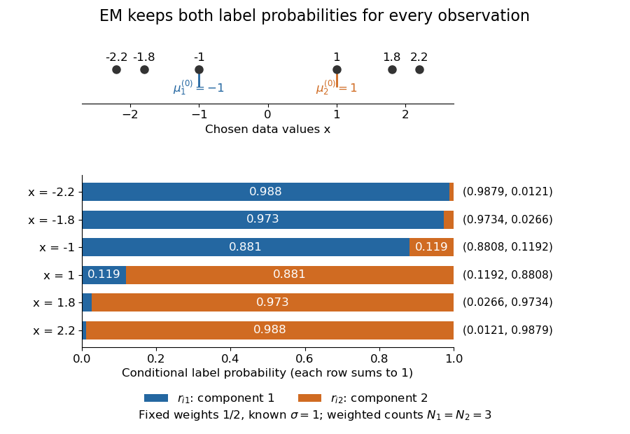

The paired values and have complementary mixture responsibilities, so exactly. The first M-step givesThe hyperbolic tangent expression follows by pairing the contributions at and . Assigning every negative value wholly to the first mixture component and every positive value wholly to the second would instead give means . Those hard assignments discard the overlap: the expectation-maximization algorithm is not the same update as K-means clustering.
The observed-data log-likelihood rises from initially to after one update and after two. Further updates approach means , with log-likelihood approximately . These values describe this initialization; EM likelihood monotonicity supplies no certificate of a global maximum.
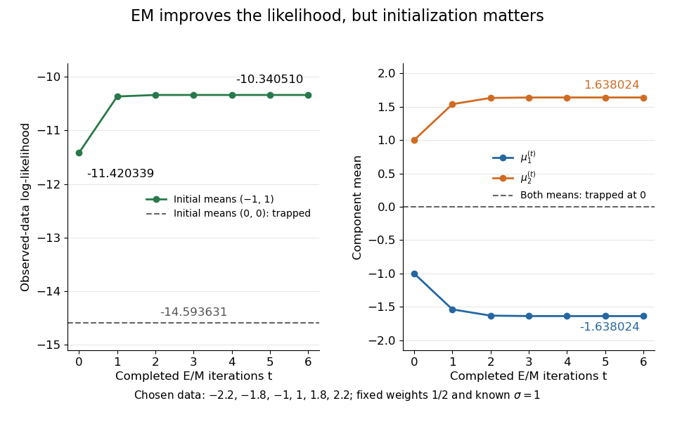
Likelihood ascent and mean updates for the chosen data, compared with an identical-means initialization
. Iteration zero is the initial fit; each subsequent point follows one E-step and one M-step. Starting at minus one and one increases the likelihood. Starting both means at zero leaves them at zero with a lower constant likelihood. All runs keep variance one and weights one half. Details.
For stable numerical evaluation, put and . The log-sum-exp function givesSubtracting keeps at least one exponential equal to one, avoiding the all-zero sum that direct evaluation of tiny component densities can produce.
In the Known-variance Gaussian mixture EM example, initialize both means at the same value . The mixture responsibilities are then for every observation. Each M-step sets both means to the sample mean, zero here; the next E-step again gives . Thus is a fixed point with log-likelihood , despite the better fit found from .
One can check the failure without trusting an iteration plot. Separate the means as and use the hyperbolic cosine identity:The Taylor expansion uses . Small nonzero separation therefore improves the log-likelihood, whereas translating both means to changes it by . This stationary point has both improving and worsening directions. Identical initialization cannot discover the separation because every observation keeps identical label probabilities. Trying several distinct initial fits and comparing their final log-likelihoods is useful, but does not prove global optimality.
Keeping the variance fixed also removes a different pathology. With known , every component probability density function is at most , so . If separate component variances are allowed to shrink without restriction, one mixture component can concentrate at an observation while another retains positive density at the other observations, making the likelihood function unbounded. The fixed positive variance in this example prevents that collapse; it does not remove initialization traps.
For observations from each of two labeled exponential distributions, an E-step may produce positive completed time totals . Its expected complete-data log-likelihood is . This is strictly concave. On the closed ordering constraint , its maximum is when ; otherwise it lies at . To see the boundary case, first maximize along the equality line. At that maximum, moving into either feasible rate-separating direction has directional derivative , so concavity proves global optimality. For the open constraint , this boundary value is a supremum rather than an attained M-step.
// Target: probability-and-statistics.bigb
For a multinomial distribution with two unobserved cells merged into one observed count, the conditional allocation is a binomial distribution with probabilities proportional to the two cell probabilities. The expectation-maximization algorithm replaces the missing counts by their conditional expectations in the parameter-dependent part of the complete-data log-likelihood. The expectation of a log-factorial normalization generally differs from its value at the expected count, but this difference is independent of the candidate parameter and does not affect the maximization step.
For independent normal coordinates, an unobserved first coordinate has conditional law equal to its current marginal normal distribution, even when the second coordinate of that observation is known. Thus its E-step first moment is and second moment is . With three observed first coordinates and one missing value, the mean update is and the variance update is . The conditional variance term is essential: filling in only the conditional mean is not the expectation-maximization algorithm.
For a common unconstrained Markov kernel on the edges of a rooted tree, let be the conditional expectation of the number of transitions , given observed leaves and the old Markov kernel. The expectation-maximization algorithm maximizes over row probability distributions, giving . A row with zero total count is unrestricted by this objective. Belief propagation computes the counts exactly on a tree.
In the expectation-maximization algorithm for a stationary autoregressive process of order one, a single missing interior value has a normal distribution conditional on its neighbors. The E-step uses both its conditional mean and its conditional second moment, not just mean imputation. The M-step maximizes the expected stationary complete-data log-likelihood, including the initial-observation density and the conditional-variance contribution to the two adjacent innovation squares.
For , the Jensen inequality givesThus any expectation-maximization algorithm M-step that increases cannot decrease the observed-data likelihood function.[ref]
For a short proof, assume common support and finite expressions, and keep the E-step conditional distribution fixed. The concavity of the logarithm and Jensen's inequality giveThis evidence lower bound equals . At , the ratio inside the expectation is the constant , so equality holds. During the M-step, the second term is constant; increasing raises a lower bound that touches the current log-likelihood. HenceIncreasing likelihood values alone do not establish convergence of the statistical parameters or attainment of a global maximum. In a differentiable finite mixture model, the gradient of equals the candidate-parameter gradient of evaluated at the current fit. Thus an interior fixed point of an exact M-step is a stationary point, which need not be a local maximum; the Identical-mean EM trap is an explicit counterexample. Small changes in log-likelihood can also occur before the means have settled, so inspecting both is useful.
Articles by others on the same topic
There are currently no matching articles.