In 1962, Leon Max Lederman, Melvin Schwartz, Jack Steinberger and collaborators distinguished muon neutrinos from electron neutrinos using a neutrino beam.[ref]
1988 Nobel Prize by Brookhaven National Laboratory. Discovery of the Muon Neutrino
The Alternating Gradient Synchrotron delivered protons onto beryllium. Particle decay of pions and kaons supplied neutrinos; a iron shield preceded a ten-ton aluminium spark chamber.[ref]
Production and detection are separate. In modern neutrino flavour notation,Shielding suppresses the daughter muon; a newly produced muon inside the spark chamber's aluminium marks an interaction.[ref]
1988 Nobel Prize by Brookhaven National Laboratory. Decay and aluminium readout
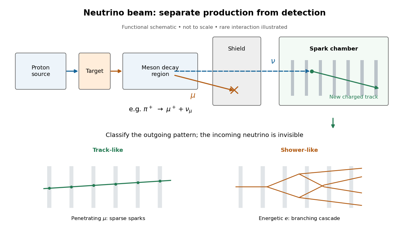

Beam-timed coincidence circuits and veto counters rejected entering tracks. Machine-off runs measured cosmic ray contamination; shield-thickness changes tested neutrons. Placing lead near the target shortened the meson decay path and reduced events. Cosmotron Electron calibration established particle shower recognition.[ref]
Observation of High-Energy Neutrino Reactions and the Existence of Two Kinds of Neutrinos by G. Danby and others. pp. 38–42, Table II, Figs. 8–9
The paper compared single-muon candidates, including estimated cosmic ray events, with six shower candidates unlike calibrated Electron showers. Kaon decays could supply genuine electron neutrinos. The deficit favored distinct neutrino flavours under lepton universality.[ref]
The inference concerns production and detection channels. It does not measure neutrino mass or establish permanently fixed neutrino flavour. Later neutrino oscillation experiments address changes during propagation.[ref]
How can the relative abundance of tracks and showers distinguish hypotheses? Consider an original teaching model, with chosen inputs throughout. Condition on a sample of selected events, each assigned exactly one of two labels: track or shower. Multitrack events and unclassified events lie outside this model. A shower label need not identify an Electron; background can imitate it. Conversely, a true Electron interaction need not receive a shower label.
Let be the background fraction among selected events. Among the selected signal events, let be the fraction whose associated charged lepton is an Electron, with the remainder associated with a muon. These are fractions after event selection, rather than fractions of the incident neutrino particle flux. Define the conditional probabilitiesHere and describe classification within the selected sample. They are not measured historical detection efficiencies. The law of total probability gives the overall shower probabilityThis formula is the bridge between an interaction hypothesis and a visible label. It keeps beam contamination, background and mistaken classification conceptually distinct: genuine electron neutrino interactions belong in , while non-signal events belong in .
Assume independent random variables for the event labels, all with this same . If counts shower labels, every specified pattern with showers has probability . Counting those patterns with a binomial coefficient yields the binomial distributionThe track count is , so its expected value is . At fixed , the two counts cannot fluctuate independently. The variance above measures sampling fluctuations under the stipulated model, not uncertainty in , , or .
Choose , , , and . Compare a signal with only muon-associated interactions () against one with equal selected Electron- and muon-associated interactions (). These give and , respectively. Their expected shower counts are and ; their expected track counts are and . A background-only model with the specified gives showers and tracks on average. These are expectations, so they need not be integers.
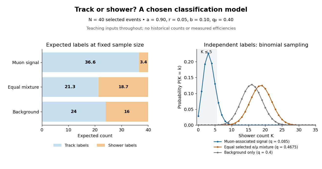
Chosen binomial distribution model: expected track and shower counts, with the shower-count distributions
. Original calculations for forty selected events and the stipulated classification and background probabilities. No historical counts, fitted efficiencies or reconstructed significance are plotted. Details.
For a hypothetical observation , the likelihood ratio of the two signal models isThe binomial coefficient cancels because the same hypothetical sample is used in both likelihoods. This ratio is not the probability that either hypothesis is true. A separate original check gives , and for the muon-associated, equal-mixture and specified background-only models, respectively.
Why are the controls essential? If the background-only model may choose any , taking can fit the observed shower fraction. Counts alone then fail to distinguish it from a signal model. Independent background measurements and calibrated particle identification constrain that freedom. Changing the decay path additionally tests where the candidate-producing particles originate. The power of the experiment comes from combining apparatus interventions with event classification; the small binomial distribution model isolates only the latter part of that reasoning.
Articles by others on the same topic
There are currently no matching articles.