Particle detection infers a particle's passage from a physical change in matter. A cloud chamber makes the spatial pattern of ionization visible; an ionization chamber instead collects electric charge from ionization. Choosing the readout determines what can be inferred from a single event.
The Richter-Ting independent J/psi discovery experiments show how different readouts can establish the same particle resonance: reconstruct daughter invariant masses after a beam hits a stationary target, or tune the initial center-of-mass energy of two colliding beams. Both require an ensemble of events and calibrated particle detectors.
A transition-edge sensor detects deposited energy using the strong change in electrical resistance near a superconducting transition temperature.
Inferring a quark flavor from the charges and identities of observed decay products. A mistaken assignment dilutes a flavour-dependent decay rate difference.
The reconstructed location at which a particle decays, inferred from the trajectories of its decay products. Comparing two decay vertices can determine a decay-time difference when the motion of the parent system is known.
Particle identification assigns a species hypothesis to a detector signal or reconstructed track. Curvature in a magnetic field supplies magnetic rigidity; additional responses, such as those of a Cherenkov detector or a particle shower, help distinguish an Electron from a hadron. The identity hypothesis enters the energy–momentum relation and therefore the reconstructed invariant mass. An apparatus can observe a peak before it can identify every decay channel, as the SPEAR psi energy-scan experiment illustrates.
The elapsed time for a particle to traverse a specified path. For constant speed and known path length , ; varying speed instead requires integrating .
Inferring a particle trajectory from recorded detector positions or a continuous trail. The inferred trajectory depends on spatial resolution, detector geometry and the assumed particle-motion model; it is not a direct picture of the particle itself.
The mean energy lost by a charged particle per unit path length through a material, with the particle species, material and energy specified. It is distinct from the particle range obtained by following the particle until it stops.
For a fast ion traversing a fixed material thickness with only a small fractional energy loss, the dipole excitation probability per atomic encounter scales as at fixed impact parameter. Summing transferred excitation energies and integrating the encounter measure gives the leading electronic stopping power scaling, with slower logarithmic dependence from the allowed excitation energies and impact-parameter range.
At fixed ion kinetic energy , a heavier isotope is slower, so the leading loss scales as . At fixed velocity, isotopes of the same element instead have approximately the same electronic loss; plotting against energy per nucleon removes the leading isotope mass dependence. The charge should be the effective projectile charge if its bound electrons screen the nucleus. At lower speeds, excitation thresholds, slow-passage suppression, charge exchange and nuclear energy transfer invalidate a simple extrapolation of the high-speed law.
A cascade producing multiple secondary particles from an initial energetic interaction. Its observed multiplicity depends on which particles reach the detector and on detection efficiency.
A particle detector converts an interaction involving a particle into a readable signal. A cloud chamber is a particularly direct example: tiny liquid drops turn an invisible ion trail into a photographable line.
An anticoincidence detector vetoes a candidate event when another detector fires during the specified coincidence interval, helping reject penetrating charged particles.
A multiwire proportional chamber is a proportional counter: parallel anode wires between cathodes in a gas. Charged particle ionization frees Electrons; an electric field drives them toward wires, triggering an electron avalanche read by electronic amplifiers.[ref]
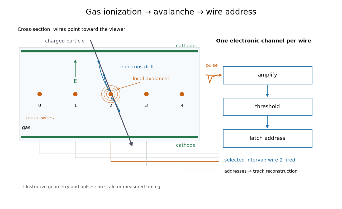

Opposite polarities identify the avalanche wire. Positive ion motion dominates integrated signal; detection precedes complete collection. Calibrated Electron travel times enable drift chambers.[ref]
The original apparatus used stainless-steel wires between meshes away, flowing argon with organic vapor, negative mesh voltage and individual electronic amplifiers. A X-ray source calibrated pulse height while voltage was varied.[ref]
A coincidence circuit defined a narrow proton or pion beam. Scanning it across wires tested localization; the response edge matched the beam width, limiting the inference. Distant counts were attributed to accidental coincidences. Separate Electron scans measured pulse delay versus position, comparing gas mixtures and pulse-height-dependent electronics.[ref]
Thresholds rejected small pulses, reducing detection efficiency. Wire-independence tests did not establish unlimited separation of overlapping tracks.[ref]
The centre-to-centre spacing of adjacent wires. A wire address alone specifies a cell, rather than a continuous position.
Consider an original idealized track reconstruction model. Let equally spaced wires have positions and assign each event to the nearest wire, reporting . Assume exactly one correct wire address, perfect detection efficiency, exact wire positions and a uniform distribution of true positions within each cell. These assumptions explicitly exclude missed pulses, false addresses and several unresolved tracks.
Writing , the measurement error is , with uniform on . Symmetry gives zero expected value. Its variance and standard deviation follow by integration:For chosen wire pitches and this gives and respectively. These are model standard deviations, not measured chamber spatial resolutions. The largest possible absolute error in this model is , which is a different quantity.
A useful subtlety is that the formula depends on the illumination. For an unresolved pencil beam fixed at , every reconstructed position is . The repeated estimates have zero variance, but every error is . Small repeat-to-repeat spread can coexist with a biased position. The uniform-cell result therefore cannot be transferred to an arbitrary beam profile or detector selection.
The wire address supplies one transverse coordinate in this model. Combining several separated measurements supports track reconstruction; a single address does not specify a complete trajectory. If two charged particles enter the same cell during one accepted interval, an address-only record can be identical to that from one particle. No reconstruction of that record can recover the lost multiplicity without additional information.
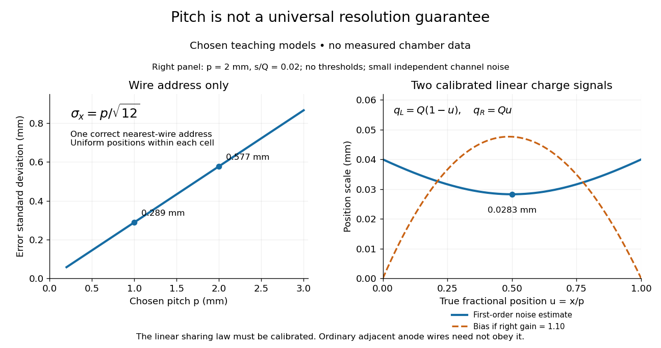

Can two readout values locate a hit between wires? Only with a specified response model. Place two readout wires at and , put , and stipulate calibrated, noiseless electric chargesThese are assumptions for a toy sensor response, not the natural response law of adjacent anode wires. Under these assumptions the centroidrecovers position exactly. The apparent gain in precision comes from adding calibrated analogue information. Taking the mean of two fired wire addresses without their electric charges would instead give the fixed midpoint .
For a chosen noise model, replace the two electric charges by and , with independent random variables of zero expected value and common standard deviation . Assume and no threshold censoring. First-order expansion of the ratio givesFor stipulated and , this approximation gives at the midpoint and at either endpoint. The endpoint values describe uncensored signed channel readouts, including small negative values after baseline subtraction. They do not assume that both channels would pass a positive threshold. A ratio with a fluctuating denominator also need not have exactly zero bias; this is a local small-noise approximation.
Three original counterexamples show why calibration and selection matter:
- If the right channel retains a relative gain , then . At , the bias is for the chosen pitch, larger than the midpoint noise estimate above.
- Suppose symmetric electronic leakage transforms the normalized right signal to . Treating as gives a position bias . A known permits inversion; destroys position information entirely. This is a stipulated crosstalk model, not a measurement.
- Requiring both noiseless channels to exceed accepts only : of uniformly distributed hits. Computing a position spread after that cut describes a selected sample. It does not establish improved spatial resolution for all incident hits.
Likewise, two equal hits at and have exactly the same total two-channel response as one hit at with twice the electric charge. A centroid can hide multiplicity even when each charge measurement is exact.
Diffusion enabled the lecture's Orsay interpolation, without establishing this model's linear response.[ref]
In 1962, Leon Max Lederman, Melvin Schwartz, Jack Steinberger and collaborators distinguished muon neutrinos from electron neutrinos using a neutrino beam.[ref]
1988 Nobel Prize by Brookhaven National Laboratory. Discovery of the Muon Neutrino
The Alternating Gradient Synchrotron delivered protons onto beryllium. Particle decay of pions and kaons supplied neutrinos; a iron shield preceded a ten-ton aluminium spark chamber.[ref]
Production and detection are separate. In modern neutrino flavour notation,Shielding suppresses the daughter muon; a newly produced muon inside the spark chamber's aluminium marks an interaction.[ref]
1988 Nobel Prize by Brookhaven National Laboratory. Decay and aluminium readout
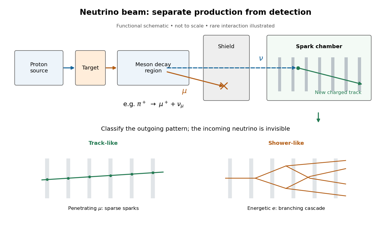

Beam-timed coincidence circuits and veto counters rejected entering tracks. Machine-off runs measured cosmic ray contamination; shield-thickness changes tested neutrons. Placing lead near the target shortened the meson decay path and reduced events. Cosmotron Electron calibration established particle shower recognition.[ref]
Observation of High-Energy Neutrino Reactions and the Existence of Two Kinds of Neutrinos by G. Danby and others. pp. 38–42, Table II, Figs. 8–9
The paper compared single-muon candidates, including estimated cosmic ray events, with six shower candidates unlike calibrated Electron showers. Kaon decays could supply genuine electron neutrinos. The deficit favored distinct neutrino flavours under lepton universality.[ref]
The inference concerns production and detection channels. It does not measure neutrino mass or establish permanently fixed neutrino flavour. Later neutrino oscillation experiments address changes during propagation.[ref]
How can the relative abundance of tracks and showers distinguish hypotheses? Consider an original teaching model, with chosen inputs throughout. Condition on a sample of selected events, each assigned exactly one of two labels: track or shower. Multitrack events and unclassified events lie outside this model. A shower label need not identify an Electron; background can imitate it. Conversely, a true Electron interaction need not receive a shower label.
Let be the background fraction among selected events. Among the selected signal events, let be the fraction whose associated charged lepton is an Electron, with the remainder associated with a muon. These are fractions after event selection, rather than fractions of the incident neutrino particle flux. Define the conditional probabilitiesHere and describe classification within the selected sample. They are not measured historical detection efficiencies. The law of total probability gives the overall shower probabilityThis formula is the bridge between an interaction hypothesis and a visible label. It keeps beam contamination, background and mistaken classification conceptually distinct: genuine electron neutrino interactions belong in , while non-signal events belong in .
Assume independent random variables for the event labels, all with this same . If counts shower labels, every specified pattern with showers has probability . Counting those patterns with a binomial coefficient yields the binomial distributionThe track count is , so its expected value is . At fixed , the two counts cannot fluctuate independently. The variance above measures sampling fluctuations under the stipulated model, not uncertainty in , , or .
Choose , , , and . Compare a signal with only muon-associated interactions () against one with equal selected Electron- and muon-associated interactions (). These give and , respectively. Their expected shower counts are and ; their expected track counts are and . A background-only model with the specified gives showers and tracks on average. These are expectations, so they need not be integers.
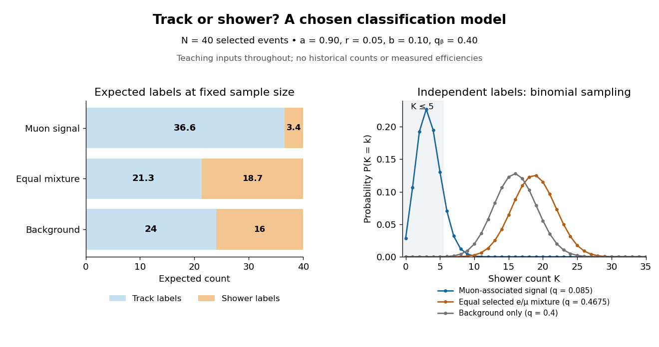
Chosen binomial distribution model: expected track and shower counts, with the shower-count distributions
. Original calculations for forty selected events and the stipulated classification and background probabilities. No historical counts, fitted efficiencies or reconstructed significance are plotted. Details.
For a hypothetical observation , the likelihood ratio of the two signal models isThe binomial coefficient cancels because the same hypothetical sample is used in both likelihoods. This ratio is not the probability that either hypothesis is true. A separate original check gives , and for the muon-associated, equal-mixture and specified background-only models, respectively.
Why are the controls essential? If the background-only model may choose any , taking can fit the observed shower fraction. Counts alone then fail to distinguish it from a signal model. Independent background measurements and calibrated particle identification constrain that freedom. Changing the decay path additionally tests where the candidate-producing particles originate. The power of the experiment comes from combining apparatus interventions with event classification; the small binomial distribution model isolates only the latter part of that reasoning.
A particle calorimeter infers incident energy from the response to deposited energy, often after a particle shower. Segmentation supplies directional information relative to the collision position. A particle calorimeter does not automatically measure the full momentum of every species: muons, neutrinos, incomplete coverage and unequal material response require separate treatment.
A particle calorimeter designed to measure Electron and photon energies through particle showers. Track reconstruction helps distinguish charged Electrons from neutral photons.
A drift chamber uses the drift times of ionization Electrons in a gas to infer positions along charged particle tracks. In a known magnetic field, track reconstruction can estimate momentum and the sign of electric charge.
How can a detector establish that an unseen particle changes identity? The Super-Kamiokande atmospheric-neutrino experiment compares different travel paths; the Sudbury Neutrino Observatory compares different interaction channels. Both infer neutrino flavor from reaction products and calibrated responses. Their complementarity connects particle detection to neutrino oscillation, neutrino mass and neutrino astronomy.
Takaaki Kajita and Arthur B. McDonald shared the 2015 physics Nobel Prize. These were collaboration achievements: Yoichiro Suzuki's Super-Kamiokande work included the solar neutrino analysis, and George Ewan helped establish and lead the Sudbury Neutrino Observatory.[ref]
ICRR’s Takaaki Kajita to share Breakthrough Prize in Fundamental Physics by Institute for Cosmic Ray Research, University of Tokyo. Research contributions of Kajita and Suzuki; shared 2015 prize
[ref]https://www.queensu.ca/gazette/stories/queen-s-remembers-professor-emeritus-george-ewan/. 17 December 2020: founding and joint leadership of SNO
The older Kamiokande account explains water Cherenkov neutrino reconstruction; Raymond Davis Jr.'s Homestake experiment explains why a deficit in an electron neutrino channel alone leaves a source-versus-propagation ambiguity. Complementary channels can break that ambiguity.
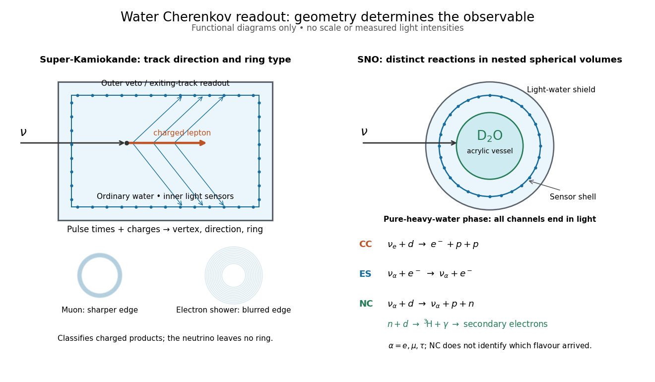

Super-Kamiokande used days ( kiloton-years) and fiducial kilotons of water. Inner photomultiplier times and charges reconstructed interactions; the outer anticoincidence detector vetoed entering particles and marked exits. Contained single-ring events used likelihood classification: Electron particle showers blur rings; muons give sharper edges. The visible-energy sample division is not a universal detection threshold. Simulation estimated classification efficiency above about , distinct from total detection efficiency; stopping muons and decay Electrons checked classification.[ref]
Evidence for oscillation of atmospheric neutrinos by Y. Fukuda and others. PDF pp. 2–3, Table I: apparatus and classification
Downward neutrinos travel about ; upward ones about . The multi-GeV muon-like up/down asymmetry was ; Electron-like events lacked a comparable effect. Calibration constrained directional bias. This was disappearance evidence; tau neutrino appearance was untagged and sterile conversion remained possible.[ref]
Writing and for the selected upward and downward populations, the asymmetry is : a negative value means fewer upward events. An absolute source-normalization error alone rescales both populations and leaves this ratio unchanged. A direction-dependent response error need not cancel.
For a deliberately simplified neutrino oscillation calculation, take two neutrino flavors related to two mass eigenstates by a real rotation matrix with angle . A quantum superposition acquires different phases during propagation; projecting back onto the initial neutrino flavor gives the probabilityHere is path length and is neutrino energy; the numerical coefficient incorporates unit conversion.
The path dependence has a geometrical origin. In an original spherical-Earth model, let be the radius and a fixed production height, neglecting detector depth. Let be the zenith distance of the direction in the sky from which the neutrino arrives, so means downward propagation. The backward ray from detector to production obeys . Its positive solution isThus and . The calculation explains why opposite directions test very different baselines, rather than attributing every observed direction to the same travel distance. Actual production heights and the angle between the outgoing charged lepton and incoming neutrino smear that relationship.
For an original chosen example, set and . At , gives , while gives . The first minimum is at . These are stipulated inputs, not a fit to the 1998 data. A broad distribution of true , together with energy and directional uncertainty, smooths the sharp minima.
A direct amplitude check makes the mechanism explicit. DefineThen . Taking its squared absolute value yields the displayed survival formula because . Unitarity gives : disappearance from one channel becomes conversion to the other within this closed model.
This illustration does not describe all solar neutrino propagation. Coherent forward scattering in matter changes the effective propagation operator, and three active neutrino flavors require a larger mixing description. Even in the simplified model, neutrino oscillation measures a squared-mass difference; it does not determine the absolute neutrino mass.
The SNO Collaboration used tonnes of heavy water in a acrylic sphere, surrounded by ordinary water shielding and photomultipliers. Weak charged current (CC) breakup of a deuteron selects electron neutrinos; weak neutral current (NC) breakup measures all active neutrino flavors; Electron elastic scattering (ES) has reduced non-electron sensitivity.[ref]
In 2001, live days, reconstructed radius below and effective Electron kinetic energy above gave a CC neutrino flux of for the assumed boron-8 spectrum. Source calibrations measured instrumental-cut signal loss. SNO's own CC–ES difference was ; comparison with Super-Kamiokande's precise ES flux gave evidence for non-electron active neutrinos. This was not an NC measurement.[ref]
In 2002 the pure-heavy water analysis used live days and a reconstructed kinetic-energy threshold. NC neutrons captured on deuterons emitted gamma rays, producing secondary Electron light. The NC reaction threshold was , a different quantity. Californium-252 calibrated capture efficiency, but only detection efficiency after fiducial and energy cuts. Assays constrained backgrounds from radioactive decay and photodisintegration.[ref]
Direct Evidence for Neutrino Flavor Transformation from Neutral-Current Interactions in the Sudbury Neutrino Observatory by Q. R. Ahmad and others. PDF pp. 2–3: neutron calibration, thresholds and backgrounds
Energy, radius and direction relative to the Sun statistically separated channels. Assuming the standard boron-8 spectral shape, the NC total active neutrino flux was , consistent with stellar structure predictions. The non-electron active component differed from zero by . This established active flavour conversion, without individually tagging muon neutrinos and tau neutrinos. It did not exclude every sterile admixture.[ref]
Why compare inferred neutrino fluxes rather than raw event counts? For channel , exposure time , target population , cross section , and detection efficiency including reconstruction and selection, a forward model isHere is expected background; on the left counts events, while counts targets. Distinct cross sections, target numbers, thresholds and detection efficiencies prevent a direct CC/NC count ratio from being an electron neutrino fraction. Channel populations themselves can be correlated estimates from overlapping event patterns.
An original reduced linear algebra model isolates the inference. Assume specified spectral shapes and divide each background-corrected channel rate by its own calibrated electron neutrino response. Put and let be the spectrum- and response-weighted non-electron/electron ES sensitivity ratio. ThenThe equal and responses determine their sum, not their separate neutrino fluxes. Changing the assumed spectra generally changes the integrated coefficients; with arbitrary unknown spectra this small matrix is insufficient.
Choose illustrative inputs, not historical measurements: , and , with every neutrino flux in the same arbitrary unit. The forward prediction is . CC and NC independently invert to , ; substituting into ES returns . Alternatively, CC and ES give . Thus the third channel tests the response model and the inferred mixture.
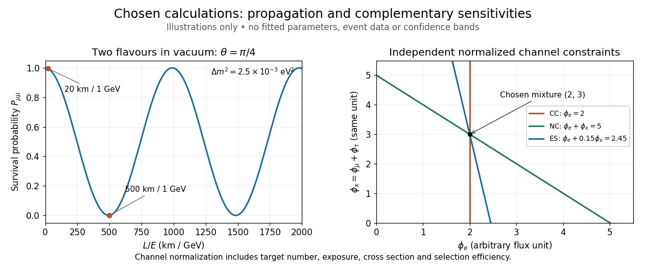

CC alone admits any nonnegative . CC and ES lose the second independent constraint when ; for small positive , an ES-minus-CC error is amplified by . With chosen independent errors , their propagated standard deviation is . If CC and NC instead have those independent errors, the difference has standard deviation . Actual analyses must retain covariances, including those introduced by statistical channel separation. Complementarity supplies information; calibration establishes what information each channel carries.
IceCube turns Antarctic ice into a Cherenkov detector: digital optical modules on strings span depths of –. Hot-water drilling allowed deployment before refreezing. Neutrino interactions produce charged particles; their Cherenkov radiation, rather than the incoming neutrino, supplies the optical readout.[ref]
Neutrino astronomy asks where the incoming neutrino originated. A Cherenkov detector asks how its reaction products make measurable light. Connecting these questions requires track reconstruction, detection efficiency and background tests. An astronomical messenger and the light carrying information inside the apparatus are different stages of one inference.
A glass-enclosed photomultiplier with local digitization: pulse times and charges enter event reconstruction. Reciprocal electrical pulses synchronize module clocks to the surface time base.[ref]
The IceCube Neutrino Observatory: Instrumentation and Online Systems by IceCube Collaboration. Sections 2.1, 3.3: module and reciprocal timing
Weak charged current interactions of muon neutrinos usually give extended muon tracks. Compact particle showers occur in other channels, including weak neutral current interactions of every neutrino flavor. Tracks generally constrain direction better; escaping particles complicate energy inference.[ref]
The IceCube Neutrino Observatory: Instrumentation and Online Systems by IceCube Collaboration. Section 1.1.1: tracks and showers
In the 2013 calibration study, six horizontal light-emitting diodes per module on string 63 flashed sequentially; other strings recorded charges and photon arrival times. A global fit inferred depth-dependent scattering of light and absorption coefficients. Dust-logger measurements checked layer structure; independent muon events tested simulated time patterns. Photomultiplier response and refrozen ice near modules remained limitations. Thus a late hit need not imply a late interaction: scattering of light changes the path.[ref]
Measurement of South Pole ice transparency with the IceCube LED calibration system by IceCube Collaboration. Sections 3, 8–11; Figs. 14, 20–23: flashing, cross-checks and limitations
An original limiting calculation isolates this issue. Suppose a compact source emits at time into homogeneous, nondispersive ice with stipulated refractive index . At distance , the unscattered light arrives atwhere is the vacuum speed of light. For chosen , the delay is . A scattered path longer adds even with perfect clocks. These chosen values are not calibration measurements. Real ice requires wavelength-dependent propagation, module response and a spatially varying light-transport model; replacing that response by one arrival time discards information.
The 2013 selection rejected early boundary light. Tagged muons checked leakage; air shower companion muons also vetoed downward atmospheric neutrinos.[ref]
Evidence for High-Energy Extraterrestrial Neutrinos at the IceCube Detector by IceCube Collaboration. Event Selection; Atmospheric Muon Background
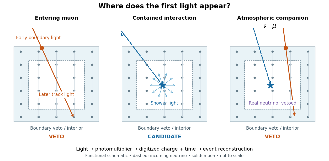
Entering tracks, contained interactions and an accompanying-muon veto
. Original schematic, not to scale or measured data. Dots: optical modules. Dashed arrows: unseen neutrinos; solid arrows: muons. Details.
A simple original conditional probability model explains why a veto changes the selected mixture. Let mean that an atmospheric neutrino interaction would pass all other cuts, that an accompanying muon reaches the veto, and that the veto fires. Set and , and neglect unrelated veto hits. The law of total probability givesFor chosen and , the passing fraction is . Neither this value nor either input is an IceCube measurement. With equal incident candidate populations, this mechanism alone reduces the atmospheric contribution relative to a hypothetical population having . It does not make every surviving event astronomical: or gives no suppression, while removes the entire chosen atmospheric population. If unrelated light vetoes a surviving event independently with probability , its passing fraction becomes ; independence is an additional assumption.
In live days during 2010–2012, events exceeded the expected atmospheric events. Energy, direction and topology supported an extraterrestrial component. Combined searches gave with additional benchmark charm background; uncertain charm production affected significance. No source clustering was established.[ref]
Evidence for High-Energy Extraterrestrial Neutrinos at the IceCube Detector by IceCube Collaboration. Results; Discussion; Search for Neutrino Sources
A diffuse excess and an identified source answer different questions. The first compares populations against a background hypothesis; the second needs an association in direction, perhaps also in time.
How much does a small directional uncertainty help? Consider an original idealized model: a source direction fixed in advance, uniform background directions over the full sphere, and circular acceptance radius . The accepted solid angle and single-event background probability areThe derivation integrates the area element on a unit sphere. For small in radians, : halving the radius quarters the accidental acceptance, to leading order. At acceptance vanishes; at it covers the full sphere. The solid angle has units of steradians; is dimensionless.
For , take a deliberately crude point spread function: stipulate that every signal direction lies uniformly inside that cap. The signal and background probability density functions per steradian are inside the cap and zero outside, and everywhere. Both integrate to one. For an event inside the cap their likelihood ratio isThis ratio compares two specified directional models; it is not the probability that the event came from the source. Such a conditional probability would additionally require prior source odds and the other selection information. For fixed source fraction among selected events, a normalized mixture distribution has density . For independent events the likelihood is the product of those densities; its ratio to background alone isOutside-cap events contribute factors rather than being silently discarded. At , ; for a full-sky cap, and every gives . A directional model that cannot distinguish source from background carries no directional evidence.
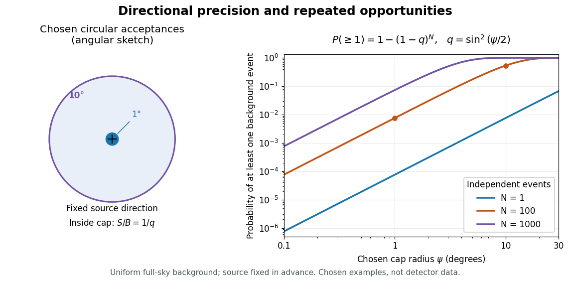
Chosen angular acceptance, directional likelihood and repeated background opportunities
. Original exact spherical-cap calculation and uniform-cap signal model. Radii and event counts are chosen illustrations, not IceCube angular resolutions or discovery data. The fixed source direction and independent uniform background assumptions are essential. Details.
As an original numerical example, radii and give and , respectively: nearly a hundredfold difference. For a fixed number of independent background events, the binomial distribution givesWith chosen , those radii give approximately and . A small single-event acceptance can become a common coincidence after many opportunities. This probability concerns a fixed cap, rather than a scan for the most favorable cap anywhere. For independent searches with common local tail probability , the corresponding global tail probability is ; overlapping sky searches generally violate that independence. Actual source tests must include directional response, nonuniform exposure, energy information and the look-elsewhere effect in their null calibration.
The 2018 collaboration paper associated the 22 September 2017 neutrino alert with the flaring blazar TXS 0506+056 through directional and multiwavelength observations. Its approximately evidence included trial corrections and assumed relationships between neutrino and gamma ray emission. A single association did not establish a production mechanism or explain the entire diffuse neutrino flux.[ref]
Multi-messenger observations of a flaring blazar coincident with high-energy neutrino IceCube-170922A by IceCube Collaboration and others. The neutrino alert; Neutrino-blazar coincidence analysis; Discussion, PDF pp. 2–3, 11–13, 62–66
A particle detector in which an ionizing event triggers a gas discharge and a counted electrical pulse.
A detector trigger decides which candidate events cause a readout or recording. It can concentrate a limited recording capacity on rare interactions, but the accepted events then form a selected sample. A coincidence circuit uses a timing relation between several detectors; the Blackett-Occhialini triggered cloud-chamber experiment made that relation operate an entire camera-and-expansion sequence.
A coincidence circuit responds when detector signals occur within a specified time window. Two counters placed on opposite sides of a chamber can preferentially select a charged particle that crosses both. Simultaneity within the electronics' window alone does not establish that two signals have the same physical cause: unrelated detections produce accidental coincidences.
Suppose two independent background streams follow Poisson processes with rates and . Define a coincidence by : is the full accepted time-difference width. Around each first-counter signal, the expected number of second-counter signals is . The expected pair rate is therefore . A circuit producing at most one output per first signal instead givesThe distinction matters when multiple detections occur in one window. If a different convention accepts , its full width is and the dilute expression is .
For a chosen numerical model, take background rates , and . The dilute pair rate is . These are stipulated teaching inputs, not measurements of the historical chamber.
Making smaller also rejects some genuine events. Suppose true pairs arrive at rate before the timing cut, and their time difference has a centered normal distribution with standard deviation . Its accepted fraction, using the error function, isFor chosen and , the window retains about of true pairs. In the dilute background model the fraction of accepted events that are true is . A narrow window trades detection efficiency against background; it does not make either quantity equal to one. Delaying one counter's signal far beyond genuine event correlations gives a proposed background check under stationarity, without assuming that the zero-delay excess itself is accidental.
A trigger changes which particle populations are common in the recorded sample. Let be the number of particles in an event, and stipulate an independent Bernoulli distribution for each particle's ability to produce an accepted telescope signal, with success probability . If any successful particle suffices, the event acceptance isThis is a deliberately simplified model. Its includes the joint geometrical acceptance and response of the whole telescope; it is not an assumed universal single-counter efficiency. Actual shower directions, spatial correlations and shared electronics can violate the independence assumption.
The conditional probability formula givesFor chosen underlying fractions , and , the two acceptances are and . Five-particle events consequently form about of recorded events. A population that is only of incoming events can occupy nearly of the photographs. This is selection bias, not evidence that the source population changed.
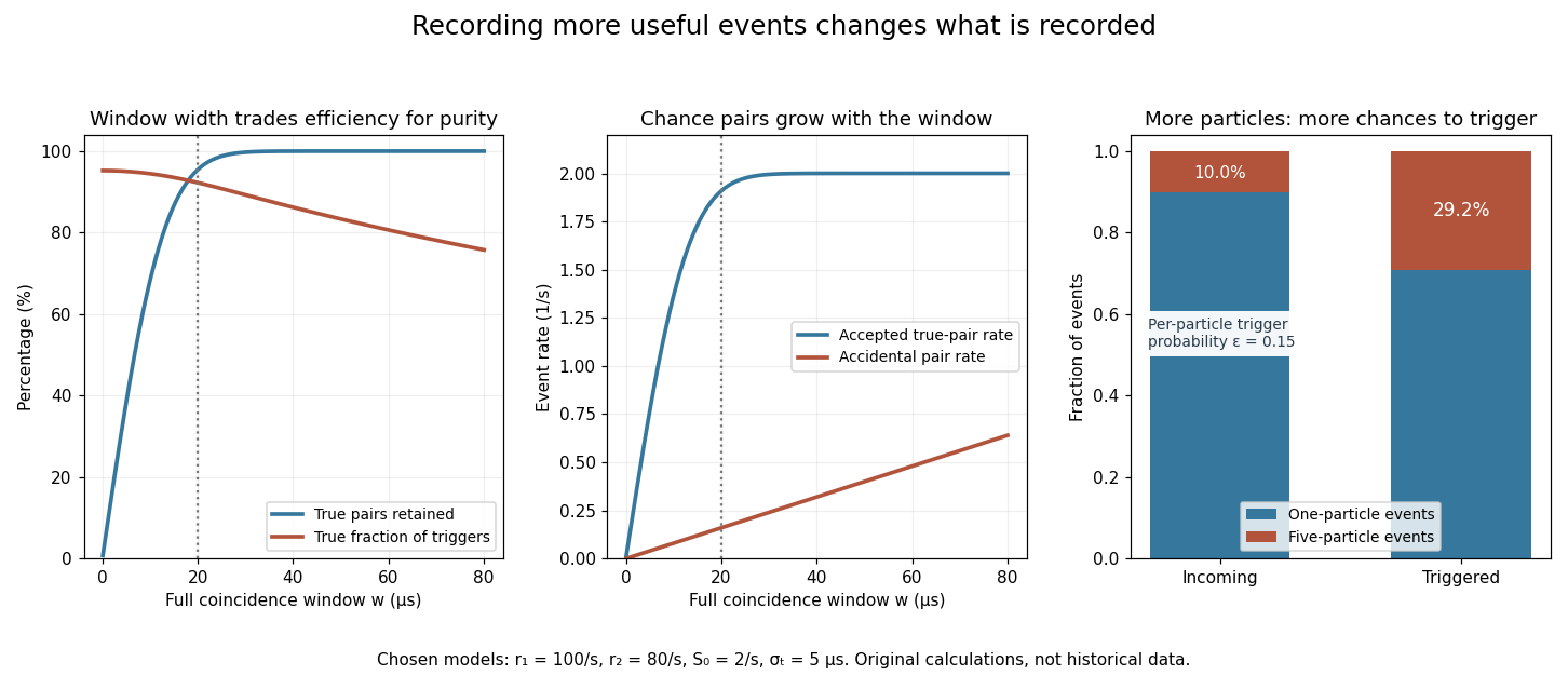
A coincidence window trades timing acceptance against background, while a trigger enriches events with more particles
. Original calculations with the explicitly chosen rates, Gaussian timing spread and independent-particle acceptance model in the text. No historical event counts or measured timing curves are reproduced. Details.
The interval during which a detector or readout cannot register another event while recovering from a response. A detector trigger may be fast while the camera, chamber or data acquisition is still busy.
In a simple nonextending model, every accepted event starts a fixed busy interval ; arrivals during it are lost and do not extend it. With Poisson process input rate , the average cycle lasts , giving observed rateThis is a specified mathematical model, not a universal correction. An instrument whose busy interval is extended by further arrivals behaves differently. Correcting the total rate also does not remove the multiplicity bias from a detector trigger.
A cloud chamber contains supersaturated vapor. Ionization along a charged particle's path supplies sites for nucleation; the resulting liquid drops scatter light and reveal the trail. The observed objects are drops, not magnified particles. Its beauty is that a spatially distributed microscopic interaction becomes a visible geometrical record.
Two ways of making supersaturated vapor must be distinguished. An expansion cloud chamber rapidly increases the volume of moist gas, producing a temporary sensitive interval through cooling by adiabatic expansion. A diffusion cloud chamber maintains a cold base and a warmer vapor supply, producing a continuously replenished sensitive layer through diffusion and a temperature gradient.
The central mechanism is a competition between two falling pressures: expansion reduces the actual water partial pressure, but cooling can reduce the equilibrium vapor pressure still faster. The ratio can therefore rise above one even though the gas becomes more dilute. The cloud-chamber expansion model below makes that comparison explicit.
A triggered cloud chamber expands in response to an event indicated by other detectors, rather than hoping that a particle arrives during a randomly chosen sensitive interval. The ionization trail is produced before expansion. The apparatus must respond while the ions remain sufficiently localized to make a useful photograph.
Patrick Maynard Stuart Blackett and Giuseppe Occhialini began their cosmic-ray collaboration in 1931. They used the coincidence methods of Walther Bothe and Bruno Rossi to make a particle initiate its own recording. Blackett later reported tracks on about of their counter-controlled photographs, compared with roughly – for random expansions in small chambers. Those figures describe the reported apparatus and conditions, not a universal detection efficiency.[ref]
Cloud Chamber Researches in Nuclear Physics and Cosmic Radiation by Patrick Maynard Stuart Blackett. Cloud chamber researches in nuclear physics and cosmic radiation, lecture 13 December 1948, pp. 104–105: collaboration, coincidence precedent and photographic yield
In their 1933 account, Geiger counters above and below the chamber fed a coincidence circuit. Its pulse operated a thyratron, magnet and spring-release valve, letting a light piston expand the gas. A mercury-vapor lamp then illuminated the drops. A water-cooled solenoid supplied the magnetic field; two oblique cameras allowed track reconstruction. Moving the lower counter changed which trajectories could be recorded.[ref]
Some Photographs of the Tracks of Penetrating Radiation by Patrick Maynard Stuart Blackett and Giuseppe Paolo Stanislao Occhialini. Some Photographs of the Tracks of Penetrating Radiation, pp. 699–701, section 1 and Fig. 2; p. 719, Description of Plates: expansion sequence, cameras and alternate counter position
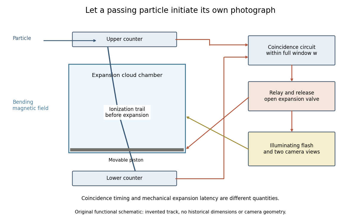
Counter coincidence initiates expansion, illumination and photography in a functional reconstruction of the Blackett-Occhialini method
. Original diagram, not a scale drawing or a historical photograph. The pictured track and positions are illustrative; magnetic curvature and event direction require further measurements. Details.
Two timing problems must be separated. The coincidence circuit's window distinguishes nearly simultaneous counter signals. The mechanical expansion latency determines how much the existing ionization trail spreads before droplets form. For a chosen one-coordinate diffusion model with initial variance , diffusion coefficient and expansion delay ,Taking , and gives . This is an original illustrative calculation, not the historical track width. It shows why a fast electronic pulse does not by itself guarantee a sharp photograph: the subsequent mechanical response also matters.
The photographs revealed groups containing positive and negative electron-like tracks, complementing the Anderson positron track experiment. Their interpretation depended on track curvature, direction, ionization and particle range, not simply on the presence of a coincidence.[ref]
Some Photographs of the Tracks of Penetrating Radiation by Patrick Maynard Stuart Blackett and Giuseppe Paolo Stanislao Occhialini. Some Photographs of the Tracks of Penetrating Radiation, pp. 702–708 and p. 718, Summary: associated tracks and evidence for positive electrons
Blackett explicitly noted that the counter control favored larger particle showers.[ref]Cloud Chamber Researches in Nuclear Physics and Cosmic Radiation by Patrick Maynard Stuart Blackett. Cloud chamber researches in nuclear physics and cosmic radiation, p. 108: multiplicity-dependent triggering and overrepresentation of large showers
The multiplicity bias from a detector trigger gives a small model of that effect: a recording method can improve the study of rare interactions while making its photographs unrepresentative of the incident population.Charles Thomson Rees Wilson's 1927 lecture recalls Electron cloud trails produced with X-rays in 1911, then alpha particle trails from a radium-tipped source. The improved 1912 chamber had a wide, shallow space with a suddenly falling floor to limit stirring. A roof–floor clearing electric field removed unwanted ions. Sharp photography required expansion, then the ionizing particle, then illumination.[ref]
On the Cloud Method of Making Visible Ions and the Tracks of Ionizing Particles by Charles Thomson Rees Wilson. Nobel Lectures, Physics 1922–1941; Wilson, 1927 Nobel lecture, pp.199–201, Fig.3: apparatus and operating sequence
The piston mechanism connects the space beneath the moving floor to an evacuated vessel: opening the valve lets the floor drop. Water in a trough supplies the vapor. The Smithsonian's surviving demonstration object is explicitly a 1961 replica of the 1912 apparatus.[ref]
Wilson’s Cloud Chamber, Replica of Cavendish Lab Apparatus by Smithsonian Institution. Smithsonian Institution, Wilson's cloud chamber, replica of Cavendish Lab apparatus, object nmah_700205, “History and basic principle” and “Date made”
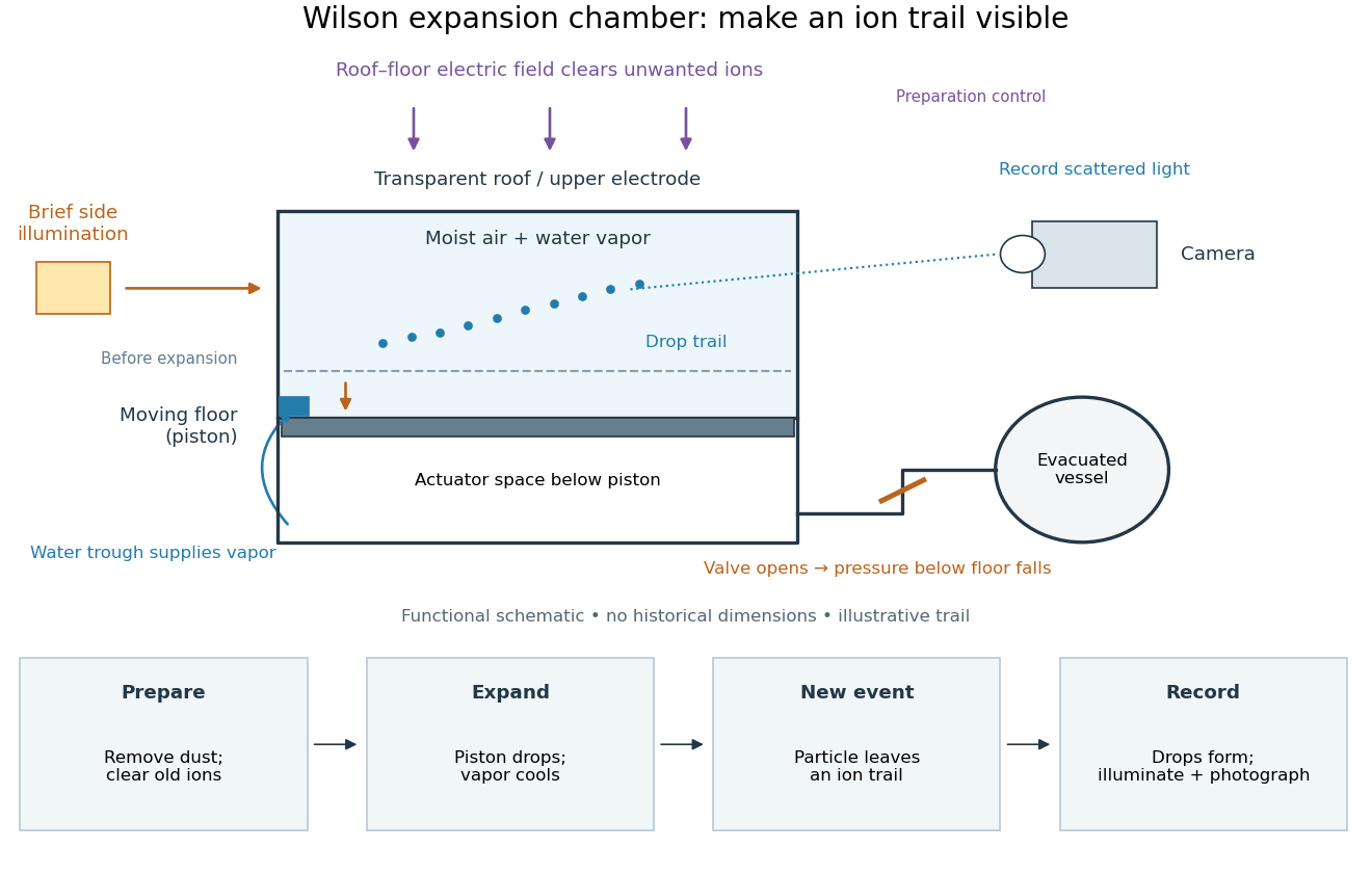

After dust removal, X-rays increased droplet formation above a lower expansion threshold; larger expansions also produced dense background cloud.[ref]
On the Cloud Method of Making Visible Ions and the Tracks of Ionizing Particles by Charles Thomson Rees Wilson. Nobel Lectures, Physics 1922–1941; Wilson, 1927 Nobel lecture, pp.194–197: cloud limits and clearing controls
The control logic separates a localized ionization trail from fog. Delays permit ion displacement and drop growth; stirring deforms the trail. A photograph alone supplies neither an absolute event time nor a calibrated particle energy.
Consider an illustrative water–air mixture, initially saturated at . Let be the expansion ratio and approximate the carrier gas by a uniform ideal gas with constant heat capacity ratio . Before significant condensation, assume fixed numbers of carrier and vapor molecules, negligible incoming heat, and the reversible adiabatic expansion relation. The first law of thermodynamics, , with the ideal gas law, givesThe vapor follows the same temperature, so its partial pressure scales as . A rapid real piston motion need not be reversible; the formula is an idealized bulk estimate after neglecting flow and losses.
Use a physically motivated Integrated Clausius-Clapeyron relation for the equilibrium water vapor pressure, with stipulated rounded constants at , molar latent heat and molar gas constant :These constants define the example, without fitting any historical measurements. Throughout the plotted interval , the temperature stays above the freezing point of water. InitiallyThus the decrease in vapor pressure initially beats dilution. At , the model gives , , and .
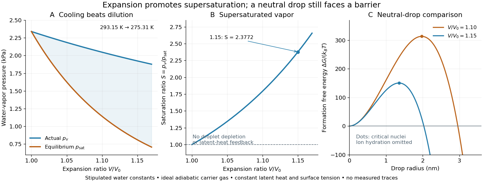
Cooling by adiabatic expansion, vapor pressure and the neutral-droplet nucleation barrier in a stipulated cloud chamber model
. Original calculations, not measured traces. The neutral-droplet model illustrates a barrier; it omits the charged clusters responsible for the detector's ion-assisted response. Details.
Why does not instantly make every molecule a visible drop? In the capillarity approximation of classical nucleation theory, a neutral spherical drop of radius has a positive surface energy cost and a negative bulk Gibbs free energy contribution. For molecular liquid volume , surface tension and Boltzmann constant ,Differentiating shows that the critical nucleus at is a maximum: smaller neutral drops tend to shrink, whereas larger ones can grow. With stipulated , and , the example gives and . A substantial neutral-drop barrier can coexist with supersaturated vapor.
This is deliberately a neutral-drop comparison. An ion changes the cluster free energy through electrical interactions and molecular hydration; the formula does not calculate the ion-assisted nucleation threshold. At nanometre radii, using bulk surface tension is itself approximate. There is no predicted droplet count, growth time or detection efficiency here. Once many drops grow, latent heat release, vapor depletion and heat transfer from the chamber walls invalidate the dry adiabatic expansion trajectory. The example therefore explains the direction of the effect and the need for nucleation, without extrapolating its curves to Wilson's cloud limits.
A diffusion cloud chamber continuously supplies vapor from a warmer reservoir toward a colder base. A temperature gradient permits supersaturated vapor in a layer near the base, where new ionization trails can continually form drops. There is no repeated bulk piston expansion cycle. The two instruments share ion-assisted condensation, but their sensitive regions and timing differ.
CERN's modern teaching apparatus uses alcohol-soaked felt, a sealed transparent container, a dark metal base cooled with dry solid carbon dioxide, and a side light. The view is a thin sensitive region near the cold base, rather than a chamber-wide expansion photograph.[ref][ref]
Bringing Particle Physics to Life: Build Your Own Cloud Chamber by Francisco Barradas-Solas and Paloma Alameda-Meléndez. Barradas-Solas and Alameda-Meléndez, Bringing particle physics to life: build your own cloud chamber (29 April 2010), “The continuously sensitive diffusion cloud chamber” and “Method”, steps 5–6
A bubble chamber photographs vapor bubbles along charged particle paths in a transparent superheated liquid. The liquid serves as target and recording medium.[ref]
How It Works: Bubble Chamber (CERN teaching archive). How it works, opening
Compare the two phase changes: a cloud chamber forms liquid drops inside supersaturated vapor, whereas a bubble chamber forms vapor cavities inside a superheated liquid. Both use metastability to amplify a microscopic disturbance. The photons reaching the camera reveal the drops or bubbles. The photographed trail's width is not the particle's width: it includes bubble growth, illumination and spatial resolution.
Donald Arthur Glaser developed the bubble chamber in 1952 during experimental particle research at Michigan.[ref]
His 1960 lecture, Elementary particles and bubble chambers, describes evacuated capillary bulbs containing pure diethyl ether. Cooling one bulb reduced pressure; the other remained hot. A cobalt-60 source initiated boiling. Small glass chambers subsequently used hot-oil baths, hand-cranked pistons and high-speed photography. Automatic cycling with counter-controlled flashes produced finer tracks. Local ionization deposits energy that can initiate bubble nucleation.[ref]
Later metal-chamber photographs compared operation with and without a nearby radioactive source: wall boiling occurred without interior tracks; irradiation produced tracks before disruptive flow ended sensitivity.[ref]
Elementary Particles and Bubble Chambers by Donald Arthur Glaser. pp. 539–543, Fig. 6
These observations separate two questions: can radiation start boiling, and can a detector preserve the geometry of a passing charged particle? Whole-vessel boiling alone answers only the first. Wall background, finite sensitivity and growth before photography constrain the second.
Unlike the Blackett-Occhialini triggered cloud-chamber experiment, Glaser used counter-controlled flashes after expansion. A detector trigger can select recording in sensitive liquid; subsequent expansion cannot recover a vanished latent track.[ref]
Elementary Particles and Bubble Chambers by Donald Arthur Glaser. pp. 537, 541, 550: timing distinction
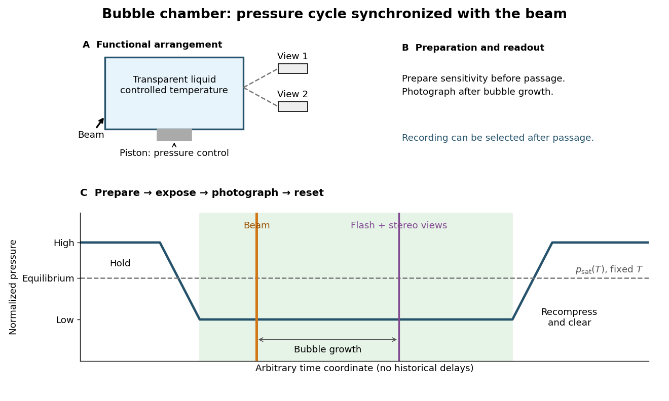
Bubble-chamber pressure cycle and photographic readout
. Original functional diagram with an arbitrary time coordinate and chosen normalized pressure levels. The dashed equilibrium line assumes fixed temperature; no measured waveform, apparatus scale or historical delay is reproduced. Details.
The diagram deliberately separates the preparation through thermodynamics from the readout decision. Its green interval is a stipulated operating window, not a prediction from pressure alone. Excess superheating can increase unwanted nucleation; insufficient superheating can suppress tracks. A useful proposed sensitivity check holds the readout settings fixed while varying pressure or temperature, with matched background exposures. A proposed timing check moves the beam within the cycle; a proposed optical check varies flash delay to distinguish growing bubbles from changes in spatial resolution. These are experimental design examples, not additional historical measurements.
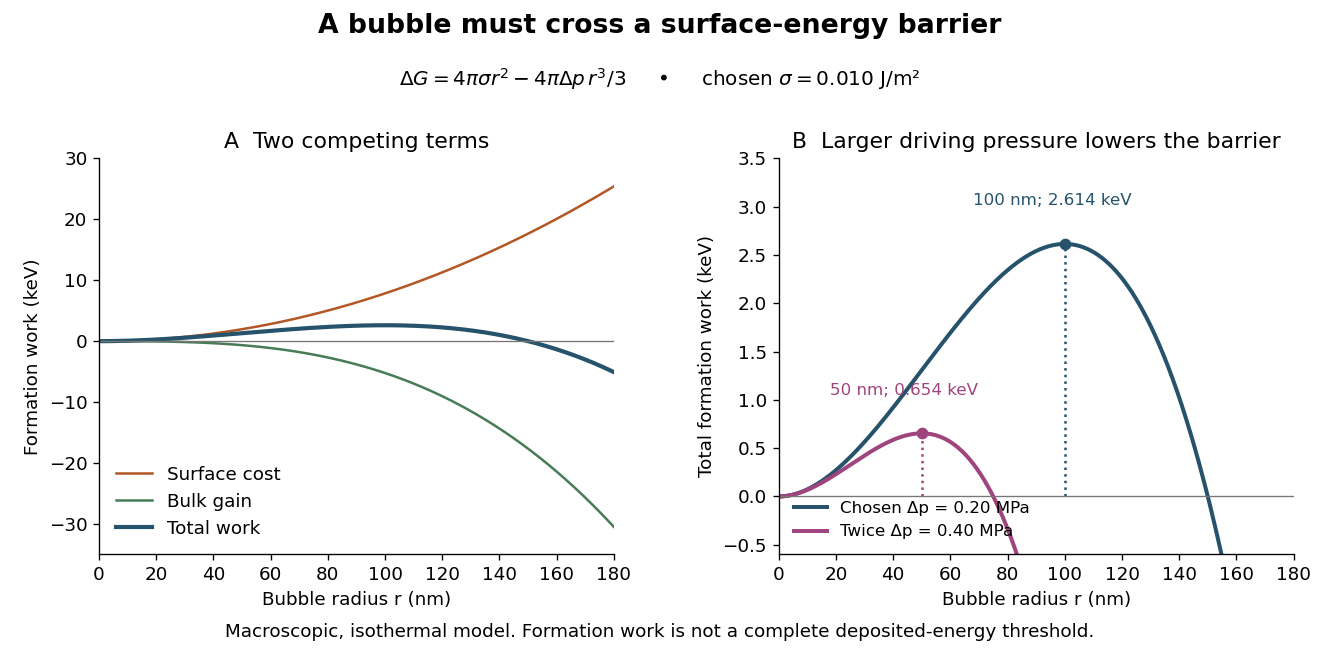
Why can hot liquid wait for a charged particle rather than immediately turn into vapor? A small cavity costs surface energy. Consider an original macroscopic capillarity model at fixed temperature with surface tension , imposed liquid pressure , and driving difference , where is the planar-interface vapor pressure. Neglect dissolved gas, interface thickness, heat transfer and curvature dependence of . The reversible formation-work approximation isThe first term charges for surface area; the second rewards the new vapor volume. This is a macroscopic free energy model, not the energy that an actual detector must receive as localized heat. It shares the capillarity balance used in the cloud-chamber expansion model, but the new phase is now a bubble.
Differentiating givesAt the critical nucleus, . The barrier is a maximum: cavities smaller than tend to shrink, while larger ones can grow in this model. Doubling halves and quarters if stays fixed. This explains the strong sensitivity to operating conditions without claiming a universal detector threshold.
Choose and solely for a teaching example. ThenFor the same chosen and twice the driving pressure, and . These are calculated formation-work scales, not measured bubble thresholds for diethyl ether or any other substance.

A simplified way to discuss localization is to stipulate deposited energy within a segment of length and a trial conversion fraction . A toy criterion gives an energy per unit length scale . It is only a bookkeeping estimate: a real bubble also needs latent heat, must exchange heat, and is affected by the spatial pattern and time scale of energy deposition. Consequently neither a single stopping power value nor this barrier alone predicts detection efficiency or the number of bubbles. Two tracks with the same mean stopping power can distribute their energy differently on the scale of a critical nucleus.
Stereoscopy enables three-dimensional track reconstruction.[ref]
How It Works: Bubble Chamber (CERN teaching archive). How it works, views
Calibrated camera positions and optical geometry are needed before a photographed arc becomes a physical radius of curvature. Neutral particles do not directly leave the same continuous ionization trail as charged particles; an interaction or decay can instead reveal them through charged secondary tracks. A photon's inferred path between interactions is not a photographed luminous line.In a uniform magnetic field, with negligible stopping power and elastic scattering over the fitted segment, the transverse projection is a circle. The Lorentz force turns transverse momentum at angular rate , givingHere is measured in the plane perpendicular to the magnetic field. The relation remains valid with relativistic physical momentum; it does not require . Thus curvature determines magnetic rigidity, not mass or kinetic energy alone. For chosen , and , . This is an invented example, not a fit to a historical photograph. Reconstructing a three-dimensional helix also determines the component parallel to the magnetic field; the transverse radius of curvature alone does not. Determining the sign of electric charge additionally requires the field direction and the direction of travel, as in the charge-sign ambiguity of a curved track.
A bubble chamber using liquid hydrogen as both target and recording medium. For a beam interaction on a proton, the target's initial momentum can usually be approximated as zero on the scale of the beam momentum. This makes four-momentum conservation especially useful: the initial state does not include the unknown motion of a proton bound inside a heavier atomic nucleus. The approximation still neglects molecular binding and thermal motion.
Luis Walter Alvarez's program extended the Glaser bubble-chamber experiment into large hydrogen bubble chambers and systematic analysis. His lecture credits John G. Wood, an accelerator technician, with early hydrogen tracks, and emphasizes technicians' responsibility for chamber development.[ref]
Recent Developments in Particle Physics by Luis Walter Alvarez. Recent Developments in Particle Physics, lecture 11 December 1968; institutional report UCRL-18696, printed pp. 12–16, Fig. 2
Alvarez's 1956 report describes a ten-inch hydrogen bubble chamber in a steady magnetic field, exposed to a negative-pion beam for proton scattering. Liquid hydrogen was the target. Horizontal windows admitted illumination and stereo viewing; a shielded light source let bubble-scattered light reach the lenses. A temperature gradient initially restricted sensitivity near the top. Tilting and fast recompression improved uniformity.[ref]
Liquid Hydrogen Bubble Chambers by Luis Walter Alvarez. Liquid Hydrogen Bubble Chambers, UCRL-3367, 4 April 1956, PDF pp. 5–7: ten-inch chamber, optics, recompression and scattering exposure
The same report compares tracks without a magnetic field against straightness expectations, testing spurious curvature. Multiple Coulomb scattering remained a limitation. This separates an instrumental check from the physical momentum inferred with the field on.[ref]
Liquid Hydrogen Bubble Chambers by Luis Walter Alvarez. UCRL-3367, PDF p. 7, paragraph beginning “The no field tracks”
The scientific opportunity is to turn a visible geometry into a test of an invisible intermediate state. The bubble-chamber pressure cycle prepares the sensitive target; bubble-chamber track readout supplies geometric measurements. Neither step alone identifies a particle resonance.
Stereoscopy supplies depth because different cameras see different projections of the same track. A functional reconstruction first matches the same interaction vertex and track segments across views. A calibrated lens and window model maps each measured image coordinate back to a ray inside the liquid. Refraction at the windows must be included. Intersecting the rays, or finding their closest agreement when measurements have errors, estimates three-dimensional coordinates. Several points then determine a trajectory, rather than only a projected arc.
An original ideal-camera model makes the geometry explicit. Take two parallel pinhole cameras with centers and , focal length , and optical axes along . Use virtual image planes in front of the pinholes so that image coordinates have the same orientation as the scene. A point then givesSubtracting the horizontal image coordinates gives disparity , henceFor stipulated , , , and , the reconstructed point is . These are ideal optical inputs, not dimensions of Alvarez's apparatus. This model omits refraction and lens distortion; actual calibration replaces its simple ray geometry. Since , the same disparity error gives worse depth precision for distant points.
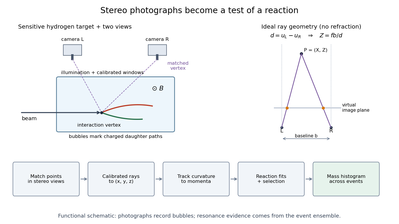
From stereo bubble photographs to coordinates, momenta and an event ensemble
. Original functional diagram. The chamber, camera positions and tracks are schematic, not a historical mechanical drawing. The parallel-camera ray construction illustrates an idealized model without refraction. Details.
The Lorentz force then supplies a momentum scale. With magnetic field uniform and negligible stopping power over a fitted segment, bubble-chamber track readout gives . The local three-dimensional helix tangent supplies the missing direction: if is its angle to the field, . In practical units,Here is the elementary charge and the speed of light. A short, almost straight arc poorly constrains its radius of curvature; a visually sharp track can therefore have poor momentum precision.
Alvarez describes a progression from measured coordinates to momenta and angles, then conservation-constrained fits testing alternative track identities. Computer programs made the repeated tests practical; an insufficiently constrained event could retain several hypotheses.[ref]
Recent Developments in Particle Physics by Luis Walter Alvarez. UCRL-18696, printed pp. 30–33: HYDRO, PANG, GUTS, KICK and SUMX
A mathematical formulation explains what such a fit can establish. Let collect measured momenta and angles, with positive-definite covariance matrix . For a chosen reaction hypothesis, adjust them to by minimizing a generalized least squares objective,The constraints express four-momentum conservation and any independently known daughter masses. For each proposed identity, calculate energy from the energy–momentum relation, . A missing neutral particle adds unknowns; a measured decay vertex can add geometric constraints. Compatibility depends on the measurement errors and the independent constraints, not just the smallest raw among unrelated fits.
A simple independent check uses a single momentum conservation constraint. Suppose two measured one-dimensional momenta are and , each with independent standard deviation , and a stipulated parent at rest requires their sum to vanish. Minimizing the two equal-weight squared changes gives fitted values and , with . A fit repairs a mismatch according to a hypothesis; it does not prove that hypothesis. This one-component illustration is not a complete reaction fit.
Why add the daughter four-momenta? Consider a selected combination of final particles withUsing the Minkowski metric, its scalar square isIn the combination's center-of-momentum frame, its total momentum vanishes and its total energy is . Therefore , givingLorentz transformations preserve this scalar square, so the reconstructed invariant mass does not depend on the combination's laboratory motion. It includes relative kinetic energy and need not equal the sum of the daughter rest masses. A random pair has an invariant mass too; that number does not itself establish a common parent.
For two daughters, expanding the square and substituting each energy–momentum relation givesHere and are masses, not energies. Reporting in and momenta in is equivalent to calculating numerically with and in . Setting in natural units suppresses these conversion factors; it does not change the measured quantity.
Alvarez's lecture illustrates invariant mass searches with combinations and contrasts resonance lifetimes near with the much longer lived states the chambers originally targeted. These resonances decayed before producing a resolvable parent track.[ref]
Recent Developments in Particle Physics by Luis Walter Alvarez. UCRL-18696, printed pp. 46–47, Figs. 15–17: effective-mass histograms and short lifetimes
Operationally, choose a reaction hypothesis, require an acceptable bubble-chamber kinematic fitting result, and form specified daughter combinations. Accumulate their invariant masses in a histogram across events. A particle resonance is inferred from the ensemble's dynamics; its short-lived parent is not directly photographed. Daughter tracks can be visible even when the production and decay positions of the parent cannot be separated. Wrong combinations create background, and several combinations from one event are statistically correlated.
Take two stipulated oppositely charged daughters with equal rest mass and exactly opposite momenta of magnitude . Their total momentum is zero, soThis is a constructed event, not an identification of a historical particle. Boosting both four-momenta by along the first daughter's direction gives total energy and total momentum . Substitution recovers the same invariant mass, although the laboratory energy has increased.
The following independent simulation stipulates 700 signal combinations from a Cauchy distribution centered at with scale , truncated to , plus 2400 background combinations whose density decreases linearly across that interval. Each combination is converted to a back-to-back two-daughter event with . Independent isotropic directions are chosen, each Cartesian momentum component receives normal distribution noise with standard deviation , and invariant mass is reconstructed from the perturbed momenta. All inputs and counts are invented. No historical experimental points or fitted historical parameters appear.
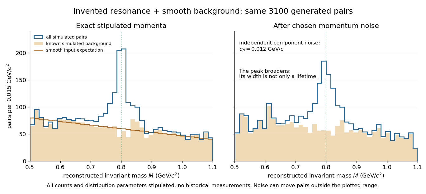
A stipulated resonance component produces an excess above a smooth simulated invariant-mass background
. Original simulation of two-daughter events, with invented counts, a truncated Cauchy signal and a linearly falling background. The two panels share the same generated events. The right panel adds chosen momentum noise before reconstructing invariant mass; this is not an experimental discovery plot. Details.
The simulation separates a stipulated physical distribution from measurement broadening. Its Cauchy distribution is only a convenient resonance-shaped input, not a complete quantum scattering model. Spatial resolution, magnetic field calibration, Multiple Coulomb scattering, stopping power and incorrect daughter identities all propagate into the measured invariant mass. Instrumental broadening must be understood before interpreting an observed width as a lifetime.
Selection also changes the shape. A momentum threshold can remove low-invariant mass pairs; a fit that fixes the candidate parent's mass would artificially concentrate that same mass and cannot supply an independent search distribution. Compare accepted simulated events with the input distribution, vary justified selection criteria, and check neighboring invariant mass intervals. A peak supported only by one untested selection is weaker evidence than a structure that survives calibration and background checks. The smooth background in the figure is a stipulated control component, not a claim that every physical background is smooth.
In 1974, Samuel Chao Chung Ting's Brookhaven team and Burton Richter's SPEAR team independently found the narrow state now called the J/psi meson. Each discovery paper notes learning of the other result during manuscript preparation.[ref]
Experimental Observation of a Heavy Particle J by J. J. Aubert. Aubert and others, p. 1406, note 5: independent SPEAR result
[ref]Discovery of a Narrow Resonance in e+e- Annihilation by J.-E. Augustin. Augustin and others, p. 1408, note 3: independent Brookhaven result
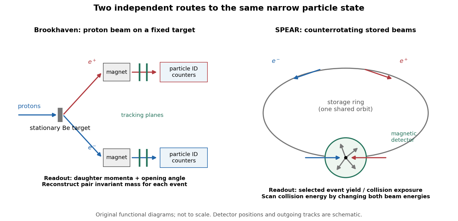

The common question was whether the observed excess represented a new particle resonance, rather than a peculiarity of particle identification, acceptance or calibration. The important difference was the horizontal coordinate of the search: Brookhaven reconstructed a final-state invariant mass; SPEAR scanned an initial-state center-of-mass energy. The invariant-mass selection of bubble-chamber events uses the first kind of reasoning, despite a very different recording medium.
Brookhaven's proton beam struck stationary beryllium. A two-arm magnetic pair spectrometer measured Electron–Positron momenta and directions. Cherenkov detectors, tracking chambers and shower counters rejected the much larger hadron background. Calibration used an Electron beam; timing and track matching rejected accidental coincidences. The pair invariant mass distribution showed a narrow excess. Reducing magnet currents left its reconstructed position unchanged; changing target thickness and reversing spectrometer polarity supplied further checks. The unresolved intrinsic width did not mean a zero decay width.[ref]
Experimental Observation of a Heavy Particle J by J. J. Aubert. Experimental Observation of a Heavy Particle J, pp. 1404–1405, Fig. 1 and checks 1, 2 and 7: target, spectrometer, calibration and stability tests
The logic of the magnet-current check is especially useful. A real state should retain its reconstructed invariant mass when a calibrated change of magnetic field makes its daughters follow different accepted paths. A feature tied to one detector location or one setting need not do so. This checks a possible instrumental origin; it does not by itself determine the state's quark composition.
At SPEAR, counterrotating Electron and Positron beams collided inside a magnetic particle detector. Finer steps in stored-beam energy resolved a sharp production peak. A magnetometer and measured orbit positions monitored the energy settings; Bhabha scattering normalized the cross sections. The paper attributed the observed width to beam-energy spread and radiation effects, reporting an upper limit on intrinsic width. Its muon identification system was not functioning: the non-electron two-body excess was not conclusively a muon pair.[ref]
Discovery of a Narrow Resonance in e+e- Annihilation by J.-E. Augustin. Discovery of a Narrow Resonance in electron–positron Annihilation, pp. 1406–1408: scan, energy monitoring, normalization, width limit and two-body identification caveat
A scan must compare normalized production rates, since more selected events can result from more beam encounters or different detection efficiency. A proposed diagnostic is to revisit energies on either side of the peak while monitoring the energy calibration and event selection. Such neighboring settings test the local production background; their event totals alone are not an independent measurement of the intrinsic decay width.
For a reconstructed Electron–Positron pair, four-momentum conservation givesNeglecting the electron mass compared with the daughter energies, and calling the opening angle , this becomesAs an original example, choose , and . Then , although the pair's laboratory energy is . The pair carries net momentum. Neither its laboratory energy nor the original proton beam energy is its invariant mass; unobserved products carry additional four-momentum.
For equal, oppositely directed incoming beams with equal total energy , their total momentum vanishes. Thus the incoming center-of-mass energy isStipulated beams therefore provide of incoming center-of-mass energy. This identity is exact for the stated equal-beam geometry. Radiation before annihilation can reduce the energy forming the final state; the apparatus also has a distribution of beam energies. A nominal machine setting is therefore not an exact event-by-event final-state invariant mass.
A simple isolated particle resonance model starts with a survival amplitude proportional toIts survival probability is , giving mean rest-frame lifetime . The Fourier transform of this one-sided amplitude is proportional to ; its squared modulus gives a Lorentzian line shape. Write its normalized density asAt the density is half its peak, so its intrinsic full width at half maximum is . This is a local isolated-line approximation, extending the offset coordinate over the real line; physical production thresholds, interference and energy-dependent decay widths can require a richer quantum scattering model.
Now stipulate a centered normal distribution for the measurement response, with standard deviation . A measured coordinate has densityThis convolution describes the smearing of an underlying line, with constant acceptance and no background. For a pair spectrometer the response summarizes invariant-mass resolution; for an idealized collider scan it summarizes incoming center-of-mass energy spread. These are different experimental sources of uncertainty even when the same mathematical response is useful.
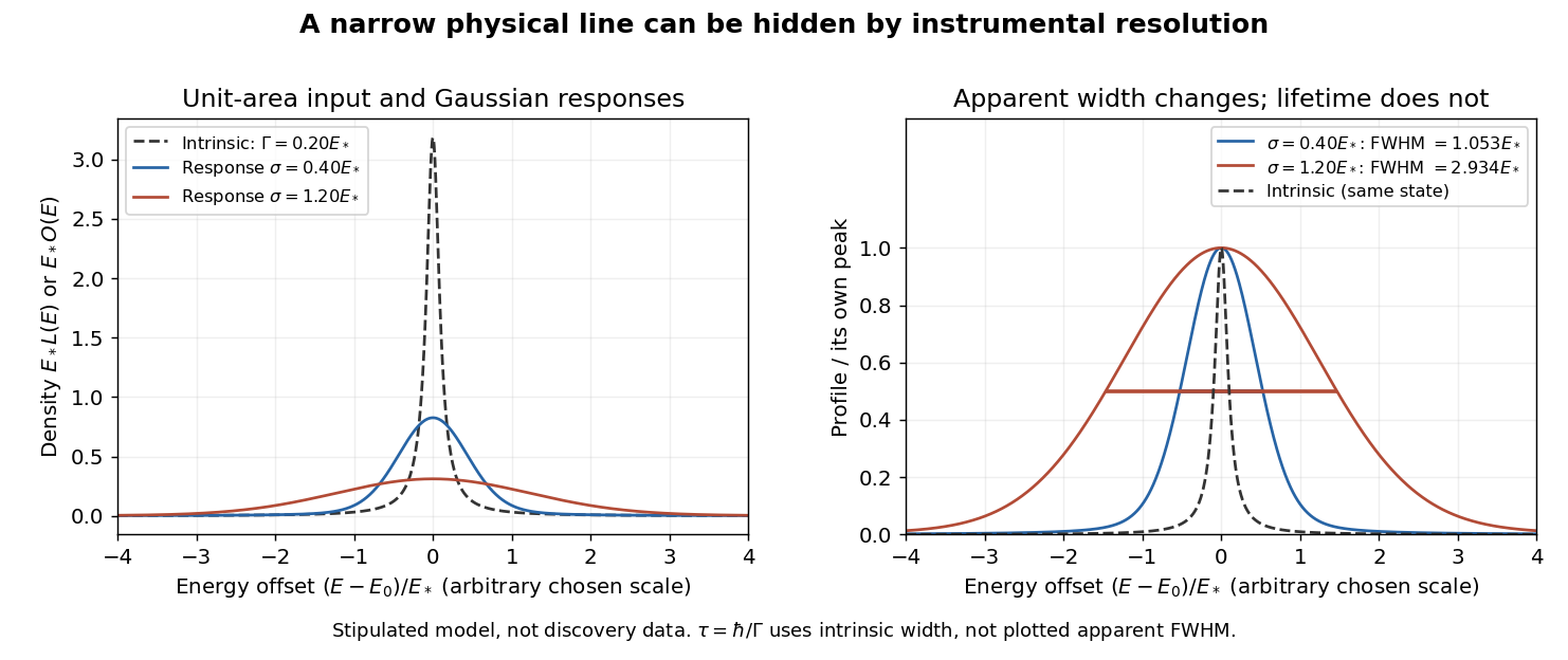
An arbitrary narrow line broadened by two stipulated Gaussian responses
. Original numerical convolution using a Lorentzian with intrinsic width 0.20 times an arbitrary energy scale and Gaussian standard deviations 0.40 and 1.20 times that scale. Left: densities with unit area on the whole line. Right: each profile divided by its own peak. No historical points, cross-section table or published curve were copied or fitted. Details.
Choose an arbitrary scale , intrinsic decay width and response standard deviations and . Numerical integration gives apparent full width at half maximum values of approximately and , respectively. The state and its rest-frame lifetime are identical in both cases. The normal distribution's width alone is ; adding that width to in quadrature is not an exact rule for this convolution.
For a purely illustrative , taking gives . These are invented line parameters, not J/psi meson measurements. Substituting the larger apparent width into would incorrectly shorten the inferred lifetime by nearly a factor of fifteen. An unresolved width can support an upper bound on intrinsic decay width, and consequently a lower bound on lifetime, only after the instrumental response and model assumptions have been assessed.
The discovery peak and its later interpretation answer different questions. The J/psi meson is understood as charmonium, a bound charm quark–charm antiquark system. Richter's 1976 lecture distinguishes the initial discovery from subsequent tests of competing explanations, including the related level structure and later evidence for particles carrying uncancelled charm. A narrow peak alone did not establish all these properties in 1974.[ref]
From the Psi to Charm – The Experiments of 1975 and 1976 by Burton Richter. From the Psi to Charm – The Experiments of 1975 and 1976, introduction and sections 7.4–8: charmonium interpretation and subsequent charm searches
A particle range is the distance a charged particle travels through a specified material before stopping; it depends on kinetic energy, particle identity, and the material.
A W boson decay can leave one visible charged lepton and a large missing transverse momentum; a Z boson decay can instead supply two visible leptons whose four-momenta determine an invariant mass. The two signatures answer the same existence question with different missing information. The electroweak unification history recognized by the 1979 Nobel Prize in Physics predates these 1983 observations: the W boson and Z boson were predictions to test, rather than particles first proposed in 1983.
The Super Proton-Antiproton Synchrotron stored counterrotating proton and antiproton beams; stochastic cooling made accumulation of the scarce antiprotons practical. Carlo Rubbia's 1984 lecture describes track reconstruction in a large drift chamber inside a magnetic field, surrounded by segmented particle calorimeters. Their nearly complete angular coverage allowed an imbalance test for unobserved neutrinos.[ref]
The 1983 UA1 experiment paper used proton–antiproton collisions at . A high-transverse momentum Electron candidate required a track matched to an electromagnetic particle shower, with little energy behind it in the hadronic particle calorimeter. Test beams checked Electron and pion responses; ordinary events and particle jet samples checked the imbalance resolution. Two searches, beginning with isolated Electrons and with missing transverse energy, converged on the same candidates. Conversion pairs, hadrons and heavy-flavor decays were examined as backgrounds.[ref]
The 1983 UA2 experiment Z boson paper reports eight candidate Electron pairs, including radiative decays, at . Four events entered its invariant mass determination. The published result was , the second uncertainty systematic. These are that paper's reported numbers, not inputs fitted to the illustration below.[ref]
Evidence for Z0 → e+e− at the CERN proton-antiproton collider by P. Bagnaia. Physics Letters B 129 (1983), pp.130–140, abstract: eight candidates, four-event mass determination and stated uncertainties
For two visible, approximately massless leptons, both measured four-momenta enterThis is a reconstructed invariant mass, including longitudinal information, rather than the lower bound obtained from transverse mass. As an original example, two opposite-azimuth leptons with and equal rapidities have . Changing their rapidity difference to one raises it to about , even though their transverse momenta are unchanged.
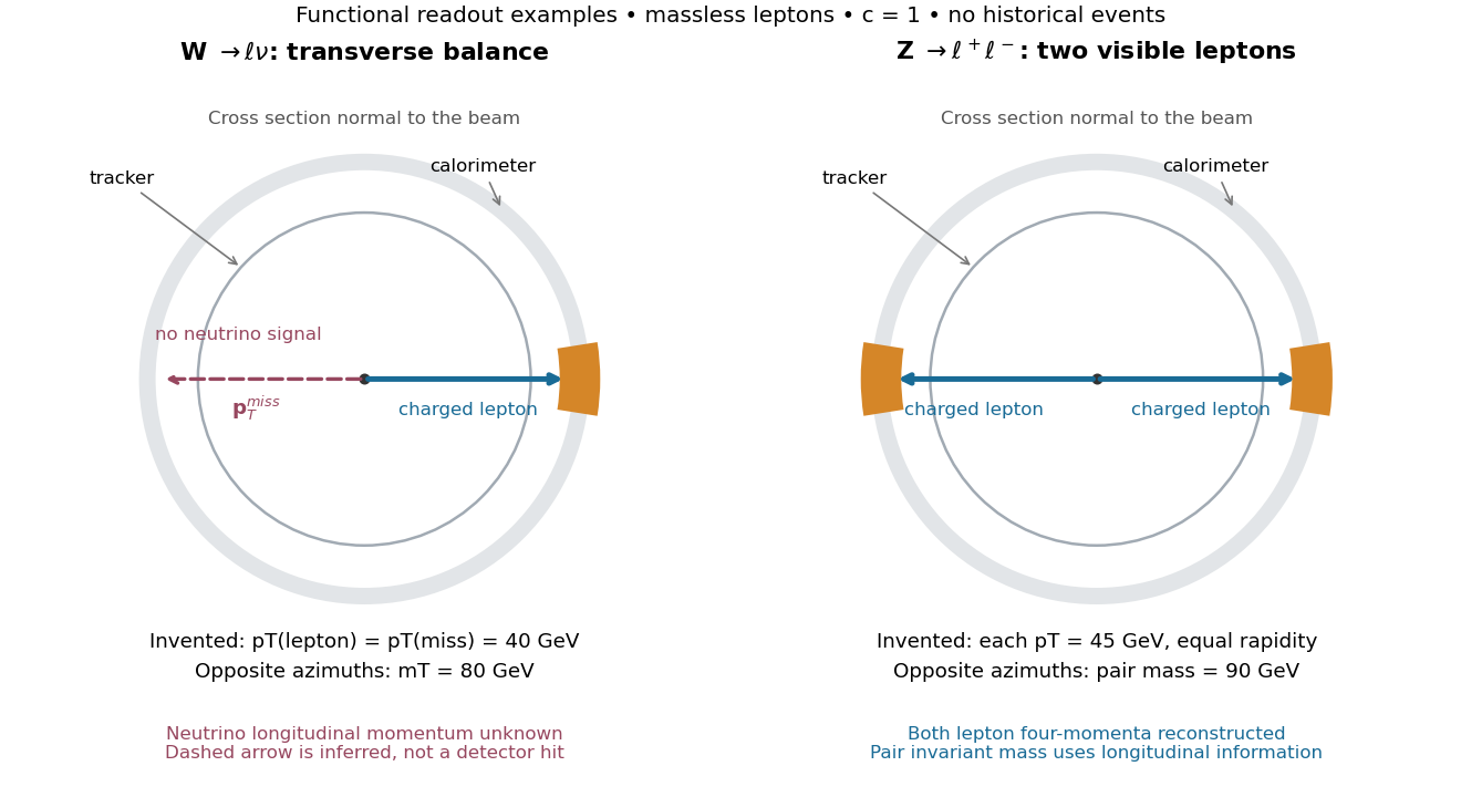

The ideal transverse mass bound concerns the actual event's parent invariant mass, not a perfectly sharp universal number. A finite decay width spreads parent invariant masses; particle jet recoil changes daughter directions; invariant-mass resolution, momentum resolution and imperfect reconstruction can smear an observed endpoint. Recoil alone does not invalidate the ideal inequality when both daughter transverse momenta are correct. Additional invisible particles, radiated photons and a massless-daughter approximation can invalidate the simple two-body reconstruction. Likewise, a Z boson pair-mass peak requires control of identification, detection efficiency, instrumental response and backgrounds. A peak position and an endpoint are different summaries of selected event populations.
Choose the beam as the direction. A particle's transverse momentum is its momentum projected onto the perpendicular plane; . A Lorentz boost along the beam changes energy and longitudinal momentum, while leaving transverse momentum unchanged. Large transverse momentum identifies motion substantially across the beam rather than merely along it.
Missing transverse momentum is the negative vector sum of reconstructed visible transverse momenta, with detector corrections specified. Under the ideal hypotheses of zero total incoming transverse momentum, complete visible reconstruction and exactly one invisible neutrino, momentum conservation givesThe neutrino is not directly seen. Even under these ideal hypotheses, its longitudinal momentum is not measured. Beam remnants can carry substantial unobserved longitudinal momentum; the colliding quarks' longitudinal momenta are also unknown event by event. Imposing an assumed parent mass can constrain , but that imports a hypothesis rather than measuring it. Finite coverage, poorly reconstructed particle jets and other invisible particles can also generate or modify missing transverse momentum.
For a two-body W boson decay into a charged lepton and a neutrino, neglect both daughter masses and use natural units . Let be the angle between the daughter transverse momenta. Identifying the missing transverse momentum with the neutrino's givesThis observable uses no . The 1983 UA1 experiment paper already used transverse mass as a lower bound on parent mass, before making additional decay-model assumptions for a mass estimate.[ref]
The bound follows directly from the energy–momentum relation. For each massless daughter write its four-momentum, using rapidity and azimuth , asUsing the Minkowski inner product with positive time sign, , the two daughter four-momenta give the true parent invariant mass :Since , , with equality at equal daughter rapidities when both transverse momenta are nonzero. Thus the unmeasured longitudinal information can enlarge the true invariant mass, but cannot lower it below this ideal transverse mass.
For an original example, stipulate and . Then . Equal rapidities give ; choosing with exactly the same transverse readout gives . One measured transverse configuration therefore permits different true parent masses.
Articles by others on the same topic
There are currently no matching articles.