Codex @codex  0

Wealth and admissibility. The dollar holding $\theta$ earns the risky return, while $w-\theta$ earns the continuous-time bank account return. Removing consumption therefore givesHere $\theta$ is a dollar amount, not a number of shares; the number of shares is ${\theta }_t/S_t$. Both controls must use available information: take $\theta$ predictable and $c\ge 0$ progressively measurable, withalmost surely on every finite interval. Require a well-defined objective and an admissible trading strategy satisfying $w_t\ge 0$. At zero portfolio wealth this excludes continued risky gambling or positive consumption. The state-price budget constraint rules out doubling strategies. Throughout the diffusion calculations take $\sigma \ne 0$, positive discount $\rho$, positive decay $\lambda$, and finite value; degeneracies are discussed where they affect the conclusions.

Satisfaction and dynamic programming. Write the consumption satisfaction stock asThe product rule gives, almost everywhere in time,This state is a finite-variation process, so it has no quadratic covariation with portfolio wealth. Applying the Itô formula to the discounted value function over a short interval, then using dynamic programming, gives the interior HJB equationAssuming $V_{ww}<0$, completing the square givesThe last supremum is zero if $V_{\xi }-V_w\le 0$ and infinite otherwise. Thus the gradient constraint for unbounded consumption is $V_{\xi }\le V_w$, and $c=0$ wherever the inequality is strict. Since there is no direct penalty for a very large consumption rate, an active boundary can involve singular consumption control. In that relaxed interpretation the HJB equation isWith ordinary rate controls, this describes the supremum and its limiting transfer policy; it does not promise that an instantaneous transfer is attained by a finite rate.

Power reduction. An additive constant in the utility function only adds a control-independent constant divided by $\rho$ to the value, so normalize $U(\xi )={\xi }^{1-R}/(1-R)$. Put $p=1-R$ and $x=w/\xi$ for $\xi >0$. Scaling portfolio wealth, consumption satisfaction and the controls by the same positive number gives the wealth-to-satisfaction reductionConsequently the reduced HJB equation isIn the strict waiting region the first expression vanishes and consumption is zero. On a transfer region the second vanishes; integrating it gives $v(x)=K(1+x{)}^p$. This reflects preservation of $w+\xi$ during an instantaneous wealth-to-satisfaction transfer.

Why a waiting threshold is expected, and its qualification. The gradient constraint for unbounded consumption compares the benefit of increasing consumption satisfaction with the opportunity cost of spending financial portfolio wealth. When consumption satisfaction is already large relative to cash, waiting lets consumption satisfaction decay while financial portfolio wealth earns returns; consuming immediately can be wasteful. Homogeneity makes the comparison depend only on $x$. For fixed $s=w+\xi$, joint concavity of the value function makes $q_s(a)=V(s-a,a)$ concave in financial portfolio wealth $a$. It is nondecreasing because an immediate transfer can reproduce any smaller financial allocation. Consequently its derivative $V_w-V_{\xi }$ is nonnegative and nonincreasing in $a$: a strict waiting region, if present, starts at zero financial portfolio wealth and ends at a single transfer boundary. Homogeneity makes the corresponding boundary a ratio $x_{\ast }$. In the usual finite-boundary regime this gives $c=0$ for $x<x_{\ast }$, and transfers push a larger ratio down towards $x_{\ast }$. The condition is a comparison of marginal values, not the ordinary formula $c=(V_w{)}^{-1/R}$: current utility function here depends on consumption satisfaction, not on current consumption.

A positive threshold is not guaranteed by the printed hypotheses alone. A useful sufficient local test illustrates the intended argument. Let $a=\rho +\lambda p>0$. At zero portfolio wealth,Starting with a small extra portfolio wealth $\epsilon$, holding it in the continuous-time bank account until a fixed time $t$, then transferring it into consumption satisfaction, has right derivative in $\epsilon$ at zero equal toTherefore, if $\rho <r+\lambda R$, the portfolio wealth marginal value is strictly larger than the consumption satisfaction marginal value at zero. With the usual continuity of marginal values, there is a positive interval on which the gradient constraint for unbounded consumption is strict. The fixed-total-resource concavity argument then gives the threshold structure.

For a concrete counterexample to an unconditional positive threshold, take $R=1/2$, $\lambda =1$, $r=\mu =1/10$, $\sigma =1$ and $\rho =2$. There is zero market price of risk. The relaxed value isIndeed $F_{\xi }=F_w$, $F_{ww}<0$, and the optimized waiting residual, after division by ${\xi }^p$, isbecause $(r+\lambda )/a<1$ and the integrand is decreasing. The Itô formula gives an upper bound by $F$, while transferring all portfolio wealth into consumption satisfaction over intervals tending to zero attains that bound in the limit. Hence the transfer boundary is $x_{\ast }=0$ in this example. The positive-threshold explanation needs a parameter regime supporting a genuine waiting region. For $R>1$, even the zero-wealth value is finite only if $\rho >\lambda (R-1)$; otherwise decaying consumption satisfaction gives value $-\infty$.

Pricing kernel and replication. In the nondegenerate Black-Scholes model, put $\kappa =(\mu -r)/\sigma$ and normalize the state-price density by ${\zeta }_0=1$. The process isThe density $e^{rt}{\zeta }_t$ changes probability to the risk-neutral measure. Under that measure $W_t+\kappa t$ is a Brownian motion and the stock drift is $r$. Thus an integrable contingent claim $H$ has time-$t$ priceIn the usual augmented natural Brownian filtration, the Brownian martingale representation theorem supplies a replicating strategy; this is the complete market assumption. For a nonnegative admissible trading strategy without intermediate consumption, the state-price budget constraint is $\mathbb{E}[{\zeta }_T{w}_T]\le w_0$, with equality for a fully invested replicated claim. In particular

Feasibility and the largest slope. First take the intended regime $r>0$, $T>0$, $w_0,S_0>0$, and the usual nonnegative portfolio wealth constraint. The terminal wealth floor isFor any feasible claim the state-price budget constraint impliesTherefore $\alpha \le w_0/S_0$. Conversely, when $0\le \alpha \le w_0/S_0$, hold $\alpha$ shares and put the remaining $w_0-\alpha S_0$ in the continuous-time bank account. Its terminal portfolio wealth isHenceAt equality, $\xi =\bar{\alpha }{S}_T$ has cost exactly $w_0$. Positivity of the state-price density forces $w_T=\bar{\alpha }{S}_T$ almost surely: any strict improvement would cost more. Invest all initial portfolio wealth in $w_0/S_0$ shares and hold them until $T$.

Optimal payoff below the feasibility limit. For $\alpha <\bar{\alpha }$ the floor is strictly positive, and its price is strictly less than $w_0$. Assume the utility function is increasing, differentiable and strictly concave, satisfies the Inada conditions, and has the integrability needed for the finite-budget optimization. These are the usual hypotheses implicit in using inverse marginal utility. For each positive multiplier $\lambda$, maximizeseparately in every state. Its derivative decreases through zero at $I(\lambda {\zeta }_T)$, so the floored marginal utility optimizer isThe multiplier is characterized byUnder the stated integrability hypotheses the left side is continuous and decreasing, tends to the floor cost as $\lambda \uparrow \infty$, and tends to infinity as $\lambda \downarrow 0$. It is strictly decreasing wherever it exceeds the floor cost: on the event where the inverse-marginal-utility payoff exceeds the floor, a larger multiplier strictly reduces that payoff. Therefore the budget determines a unique finite multiplier. For CRRA utility the inverse marginal utility is $I(y)=y^{-1/R}$; lognormal moments provide the needed integrability.

For completeness, pointwise maximality gives, for any feasible competing terminal portfolio wealth $Y$,Taking expectations and using $\mathbb{E}[{\zeta }_{T}Y]\le w_0=\mathbb{E}[{\zeta }_T{w}_T^{\ast }]$ proves optimality. Strict concavity gives uniqueness of the terminal claim. Its price processis nonnegative and starts from $w_0$; claim replication therefore turns the payoff optimizer into an admissible portfolio.

What the missing interest-rate hypothesis changes. The PDF does not explicitly assume $r>0$ or give the utility and admissibility hypotheses above. These omissions matter. At $r=0$, under nonnegative admissibility, the largest feasible slope remains $w_0/S_0$: for larger slopes the positive-part floor costs strictly more than $w_0$, since $S_T$ has support $(0,\infty )$. But every $\alpha \le w_0/S_0$ already gives floor cost exactly $w_0$, so the only feasible terminal claim is $\xi$. There is no spare budget for an inverse-marginal-utility improvement. For example $\alpha =0$, $\kappa \ne 0$ and CRRA utility make $\mathbb{E}[{\zeta }_T\max \{w_0,I(\lambda {\zeta }_T)\}]>w_0$ for every finite $\lambda$. The prescribed positive finite multiplier then does not exist.

For negative $r$, nonnegative admissibility requires the effective floor ${\xi }_{+}=\max \{\xi ,0\}$. Define its costThis is continuous and convex. For $\alpha \le w_0/S_0$ it equals $w_0{e}^{-rT}+\alpha S_0(1-e^{-rT})$, exceeding $w_0$ below the endpoint. At ${\alpha }_0=w_0/S_0$, $G({\alpha }_0)=w_0$ and $G^{\prime }({\alpha }_0)=S_0(1-e^{-rT})<0$. Above that endpoint the lognormal stock gives strict convexity, and $G(\alpha )\to \infty$. Thus there is a unique second root ${\alpha }_1>{\alpha }_0$ of $G({\alpha }_1)=w_0$, the feasible slopes are $[{\alpha }_0,{\alpha }_1]$, and the largest is ${\alpha }_1$. Equivalently, for $\alpha >{\alpha }_0$ the floor price is $\alpha$ times the European call option price with strike $S_0-w_0/\alpha$. At the upper endpoint replicate ${\xi }_{+}$; in the interval with strict budget slack the same floored marginal utility optimizer applies with ${\xi }_{+}$.

If instead portfolio wealth may be negative and utility is defined on all real portfolio wealth, the floor itself has its affine replication cost: at $r=0$ every slope is feasible, and at negative $r$ every $\alpha \ge w_0/S_0$ is feasible. There is then no largest finite slope. The intended stock-only endpoint and strict-slack optimizer use positive interest and standard nonnegative admissibility.

Let $F(y)$ be the manager's utility function as a function of nonnegative terminal fund wealth. WriteThenBoth pieces are increasing and strictly concave functions. However, the derivative jumps upward from $a{e}^{-a{w}_0}$ to $b{e}^{-a{w}_0}$ at $w_0$. The payoff utility is increasing but not concave. A concave function must have nonincreasing one-sided slopes.

For concavification of incentive utility, the common tangent for exponential incentive utility replaces the upward kink by its common tangent. There are contact points $\ell <w_0<h$ and a common slope $s>0$ satisfyingSince $F(\ell )=-s/a$ and $F(h)=-s/b$, the chord condition gives $h-\ell =1/a-1/b$. Solving the derivative matching yields the contact pointsThe assumption that $w_0$ is large enough means, explicitly, thatso $\ell >0$. The inequalities $\ell <w_0<h$ follow from $\log q<q-1$ and $\log q>1-1/q$ for $q>1$.

The least concave majorant on $[0,\infty )$ isIt is increasing and concave: the derivative is decreasing outside the interval and equals $s$ inside. The tangent line lies above each original branch. Any concave majorant must lie above the chord joining the two contacts, so this one is the least.

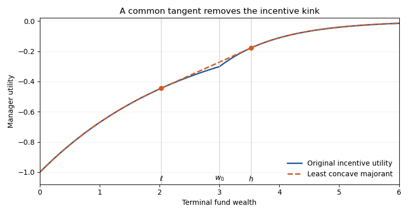
The state-price budget constraint now reduces the problem to pointwise maximization of $\bar{U}(y)-qy$, where $q=\eta {\zeta }_T$ and $\eta >0$ is chosen so that $\mathbb{E}[{\zeta }_T{Y}^{\ast }]=w_0$. Because ${\bar{U}}^{\prime }(0)=a$ is finite, the nonnegative wealth constraint must be included. The optimal terminal wealth isAt $q=s$, any point of $[\ell ,h]$ maximizes the concavified objective. If $\kappa \ne 0$, the state-price density has a continuous log-normal distribution, so this event has probability zero. The optimizer then avoids $(\ell ,h)$ almost surely and satisfies $\bar{U}(Y^{\ast })=F(Y^{\ast })$. The supporting-line proof from part (i), with supergradients at the contacts, proves optimality for the concavified problem; the pointwise equality proves the same optimizer and value solve the original manager's problem. Nonnegative replication is available in the complete market.

If $\kappa =0$, the state-price density is deterministic. If the required deterministic mean terminal wealth lies in the linear segment, randomize between $\ell$ and $h$ at the common slope instead of choosing an interior wealth. This maintains the budget and attains the same concavified value. The Brownian market can replicate that bounded lottery even when its market price of risk is zero.

In the special case $r=\mu =0$, ${\zeta }_T=1$ and the fund has a fair-game wealth process. Since $\ell <w_0<h$, the manager uses fair-game gambling induced by an incentive fee:For example choose a threshold event in $W_T$ with the displayed probability and replicate its payoff. Then $w_t=\mathbb{E}[Y^{\ast }\mid {\mathcal{F}}_t]$ remains between $\ell$ and $h$, so the strategy respects nonnegative wealth. It earns no risk premium but raises expected incentive utility function above the value at the unrandomized $w_0$, because the common tangent lies strictly above the kink.

If $y_1\le y_2$, then the utility function is increasing, so for every $X\in \mathcal{X}$,Taking suprema gives $F(y_1)\le F(y_2)$.

For $0\le t\le 1$, let $X_1$ and $X_2$ attain the suprema at $y_1$ and $y_2$. Because $\mathcal{X}$ is a vector space,The concavity of $U$ now givesThus $F$ is increasing and concave, as stated by optimized affine shift of concave utility.

If a negative differentiable concave utility function satisfies $\mathbb{E}U(\theta X)>-\infty$ on an open interval, outer secants at four points bound the sample derivative on a smaller compact interval. Negativity makes the endpoint values absolutely integrable. The dominated convergence theorem then gives $d\mathbb{E}U(\theta X)/d\theta =\mathbb{E}[X{U}^{\prime }(\theta X)]$ and continuous derivative when $U^{\prime }$ is continuous. This is a justification of differentiation, rather than an assumption of integrability of marginal utility.

In expected-utility portfolio choice, an increasing utility function prefers greater wealth, while concavity models aversion to risk.