Waveguide cutoff frequency (${\omega }_{mn}=c\pi \sqrt{m^2/a^2+n^2/b^2}$)

The waveguide cutoff frequency separates oscillatory axial propagation from exponential decay for a particular normal mode. For the vacuum-filled rectangular electromagnetic waveguide, the dispersion relation isFor a transverse electric mode of a rectangular waveguide, $m,n$ are nonnegative integers but not both zero. For a mode with $B_z=0$ and nonzero $E_z$, both indices must be positive. The lowest cutoff for $a>b$ is consequently ${\omega }_{10}=\pi c/a$, or ordinary frequency $f_c=c/(2a)$.

A square cross-section instead gives equal ${\mathrm{TE}}_{10}$ and ${\mathrm{TE}}_{01}$ cutoffs. The absence of a transverse electromagnetic mode is specific to this hollow pipe, rather than all electromagnetic waveguides.^[ref]

For $\omega >{\omega }_{mn}$, choose real $\beta >0$ for propagation toward $+z$. For $0<\omega <{\omega }_{mn}$, a field decaying into a semi-infinite guide hasA finite section can contain both growing and decaying axial solutions set by its two ends; the single decaying solution is not a complete finite-section transmission calculation. At exact cutoff $\beta =0$, the two axial solutions become a constant and a linear function of $z$: there is no finite axial wavelength for a traveling sinusoid.

In the chosen $a=30\mathrm{mm}$ guide at $f=0.8f_c=3.99723277\mathrm{GHz}$, the ${\mathrm{TE}}_{10}$ branch has $\alpha =20\pi {\mathrm{m}}^{-1}$. Its amplitude decay length is $1/\alpha \simeq 15.9155\mathrm{mm}$; after $50\mathrm{mm}$, its normalized wave amplitude is $e^{-\pi }\simeq 0.0432139$. This is geometric evanescence even with ideal walls, not Joule heating. A single decaying branch has zero cycle-averaged axial Poynting vector: substituting $\beta =i\alpha$ makes $B_x$ a quarter-cycle out of phase with $E_y$. Coupling across a finite section requires the complete boundary-value solution.

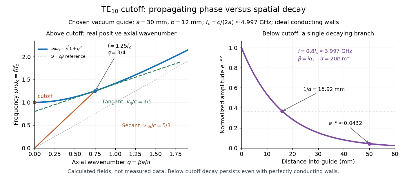
For a propagating branch of an ideal vacuum-filled rectangular electromagnetic waveguide, the phase velocity tracks constant wave phase along the axis, whereas the group velocity describes a sufficiently narrow, weakly distorted wave packet. Using ${\omega }^2=c^2{\beta }^2+{\omega }_c^2$ givesThus $v_{\mathrm{ph}}>c$, $0<v_g<c$, and $v_{\mathrm{ph}}{v}_g=c^2$. Differentiating the dispersion relation proves the second formula; dividing it by ${\beta }^2$ proves the first. This is the same mathematical structure as Klein-Gordon packet velocities. In the stipulated $f=1.25f_c$ example,Over $0.30\mathrm{m}$, the corresponding narrow-envelope delay is $(0.50\mathrm{m})/c$, approximately $1.668\mathrm{ns}$. Timing a carrier wave crest would give $0.6004\mathrm{ns}$; it does not time the arrival of a newly introduced message.

There is an independent energy check. For the forward ${\mathrm{TE}}_{10}$ fields, the average axial Poynting vector is $⟨S_z⟩=\beta |E_y{|}^2/(2{\mu }_0\omega )$. Integrating across the guide gives average power $P$ and average electromagnetic energy per unit length $U^{\prime }$:The transverse sine and cosine squared each integrate to $a/2$; ${\beta }^2+(\pi /a{)}^2={\omega }^2/c^2$ then makes the integrated electric and magnetic contributions to $U^{\prime }$ equal. The axial energy transport therefore agrees with the group velocity in this ideal model.

As $\omega \downarrow {\omega }_c$, $v_g\to 0$ and $v_{\mathrm{ph}}\to \infty$; exactly at cutoff $\omega /\beta$ is undefined. Strong wave dispersion close to cutoff also limits the narrow-packet approximation. Neither a large phase velocity nor a pulse peak establishes superluminal information velocity; front velocity asks a separate causal question. In a uniform filling with constant positive permittivity $\epsilon$ and magnetic permeability $\mu$, replace $c$ by $u=1/\sqrt{\epsilon \mu }$, giving $v_{\mathrm{ph}}{v}_g=u^2$. Frequency-dependent material response or significant loss requires differentiating the actual dispersion relation, so this product is not universal.