The "rare disease assumption" typically refers to certain underlying principles or guidelines that govern the research, diagnosis, treatment, and policy-making surrounding rare diseases. In a general context, a rare disease is often defined as one that affects a small percentage of the population, with specific thresholds varying by country.
The list of Greek mathematicians includes many influential figures from ancient Greece who made significant contributions to mathematics, geometry, astronomy, and related fields. Here are some notable Greek mathematicians: 1. **Thales of Miletus (c. 624–546 BC)** - Considered one of the first mathematicians, he is known for his work in geometry and is often credited with the first mathematical proofs. 2. **Pythagoras (c.
The Jupiter trojans are a group of asteroids that share an orbit with the planet Jupiter, residing in the two stable Lagrange points 60 degrees ahead of and behind Jupiter in its orbit. These two groups are known as the "Greek camp" (leading group) and the "Trojan camp" (trailing group). The Jupiter trojans are named after characters from the Trojan War.
Here’s a list of notable mathematics education journals you might find useful: 1. **Journal for Research in Mathematics Education (JRME)** - A leading journal focused on the research in mathematics education. 2. **Mathematics Education Research Journal (MERJ)** - Publishes original research on mathematics education. 3. **Educational Studies in Mathematics** - Covers research and scholarly discussions in the field of mathematics education.
The list of minor planets numbered 1 through 1000 consists of various small celestial bodies that orbit the Sun, primarily in the asteroid belt between Mars and Jupiter. These celestial bodies are cataloged by their official designations, which are usually assigned as they are discovered. Here are some notable minor planets from the range of 1 to 1000: 1. **1 Ceres** - The first and largest asteroid discovered, now classified as a dwarf planet.
The minor planets numbered 131001 to 132000 are part of a catalog of asteroids and other small celestial bodies in our solar system. Each minor planet is assigned a unique number for identification. These minor planets include a variety of objects with different characteristics, such as composition, size, and orbit.
The list of minor planets between 142001 and 143000 includes various small celestial bodies that are part of our solar system. Each minor planet is typically designated by a unique number and often has a name. These minor planets can include asteroids from the asteroid belt, objects from the Kuiper belt, and other distant bodies.
The list of minor planets numbered from 179001 to 180000 consists of a range of small celestial bodies, often referred to as asteroids, that orbit the Sun. These minor planets have been cataloged and numbered by the International Astronomical Union (IAU) as they were discovered. Each minor planet has a unique number and often a name or designation, which may reflect a variety of themes, such as mythology, geography, notable people, or astronomers.
The list of minor planets numbered between 182001 and 183000 is part of a large catalog of minor planets (or asteroids) that have been discovered and assigned identification numbers. Each minor planet has a unique number along with other attributes such as their names, discovery dates, and characteristics.
The list of minor planets from 200001 to 201000 includes various celestial objects that are categorized as minor planets or asteroids. These minor planets are typically small rocky bodies that orbit the Sun, primarily in the asteroid belt between Mars and Jupiter, but they can also be found in other regions of the solar system. Each minor planet is assigned a unique numerical designation upon discovery, along with a provisional designation that usually includes the year of discovery.
The List of minor planets from 222001 to 223000 includes a variety of asteroids that have been cataloged. Each minor planet is typically designated with a sequential number following the establishment of its discoverers and their respective observations.
The list of minor planets from 225001 to 226000 includes various small celestial bodies that orbit the Sun, typically in the asteroid belt between Mars and Jupiter, although some may also have orbits that take them closer to Earth or into the outer reaches of the solar system. These minor planets are designated with specific numbers in the sequence of discoveries, and many of them may have been named after people, places, or concepts.
A rectified prism, often encountered in geometry and optics, is a projection technique related to polygons and polyhedra. It is formed by truncating or "slicing off" the vertices of a prism, typically resulting in a shape that retains the characteristics of the original prism but has its corners smoothed out. In the context of optics, a rectified prism might refer to a type of optical device designed for specific light manipulation, such as reflecting or refracting light.
A numeral system is a writing system for expressing numbers; it is a mathematical notation for representing numbers of a given set, using digits or other symbols in a consistent manner. There are many numeral systems in use throughout history and across cultures. Here’s a list of some of the most significant numeral systems: 1. **Decimal (Base-10)**: The most widely used numeral system, based on ten digits (0-9).
The list of minor planets, specifically those numbered from 24001 to 25000, consists of various small celestial bodies that orbit the Sun. These minor planets include asteroids, many of which can be found in the asteroid belt between Mars and Jupiter, as well as those in other regions of the solar system.
The list of minor planets numbered 245001 to 246000 includes various small celestial bodies, primarily asteroids, that have been cataloged by the International Astronomical Union (IAU). Each minor planet is assigned a unique number, which indicates the order in which they were discovered and cataloged.
The list of minor planets numbered 260001 to 261000 consists of a series of small celestial bodies, also known as asteroids, that have been assigned a unique number by the International Astronomical Union (IAU) upon discovery. Each minor planet can have its own name, orbital characteristics, and other scientific data.
The list of minor planets numbered from 26001 to 27000 includes a variety of small celestial bodies that orbit the Sun. Each minor planet is assigned a number upon its discovery and is often given a name that may reflect a person, place, or concept associated with its discoverer or the astronomer community.
Pinned article: Introduction to the OurBigBook Project
Welcome to the OurBigBook Project! Our goal is to create the perfect publishing platform for STEM subjects, and get university-level students to write the best free STEM tutorials ever.
Everyone is welcome to create an account and play with the site: ourbigbook.com/go/register. We belive that students themselves can write amazing tutorials, but teachers are welcome too. You can write about anything you want, it doesn't have to be STEM or even educational. Silly test content is very welcome and you won't be penalized in any way. Just keep it legal!
Intro to OurBigBook
. Source. We have two killer features:
- topics: topics group articles by different users with the same title, e.g. here is the topic for the "Fundamental Theorem of Calculus" ourbigbook.com/go/topic/fundamental-theorem-of-calculusArticles of different users are sorted by upvote within each article page. This feature is a bit like:
- a Wikipedia where each user can have their own version of each article
- a Q&A website like Stack Overflow, where multiple people can give their views on a given topic, and the best ones are sorted by upvote. Except you don't need to wait for someone to ask first, and any topic goes, no matter how narrow or broad
This feature makes it possible for readers to find better explanations of any topic created by other writers. And it allows writers to create an explanation in a place that readers might actually find it.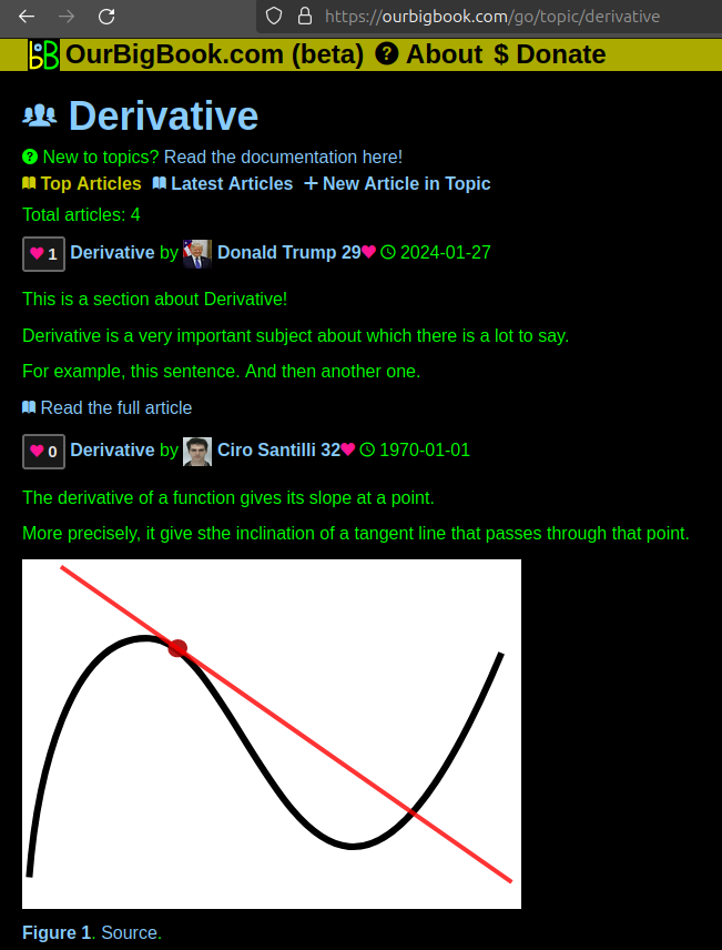
Figure 1. Screenshot of the "Derivative" topic page. View it live at: ourbigbook.com/go/topic/derivativeVideo 2. OurBigBook Web topics demo. Source. - local editing: you can store all your personal knowledge base content locally in a plaintext markup format that can be edited locally and published either:This way you can be sure that even if OurBigBook.com were to go down one day (which we have no plans to do as it is quite cheap to host!), your content will still be perfectly readable as a static site.
- to OurBigBook.com to get awesome multi-user features like topics and likes
- as HTML files to a static website, which you can host yourself for free on many external providers like GitHub Pages, and remain in full control
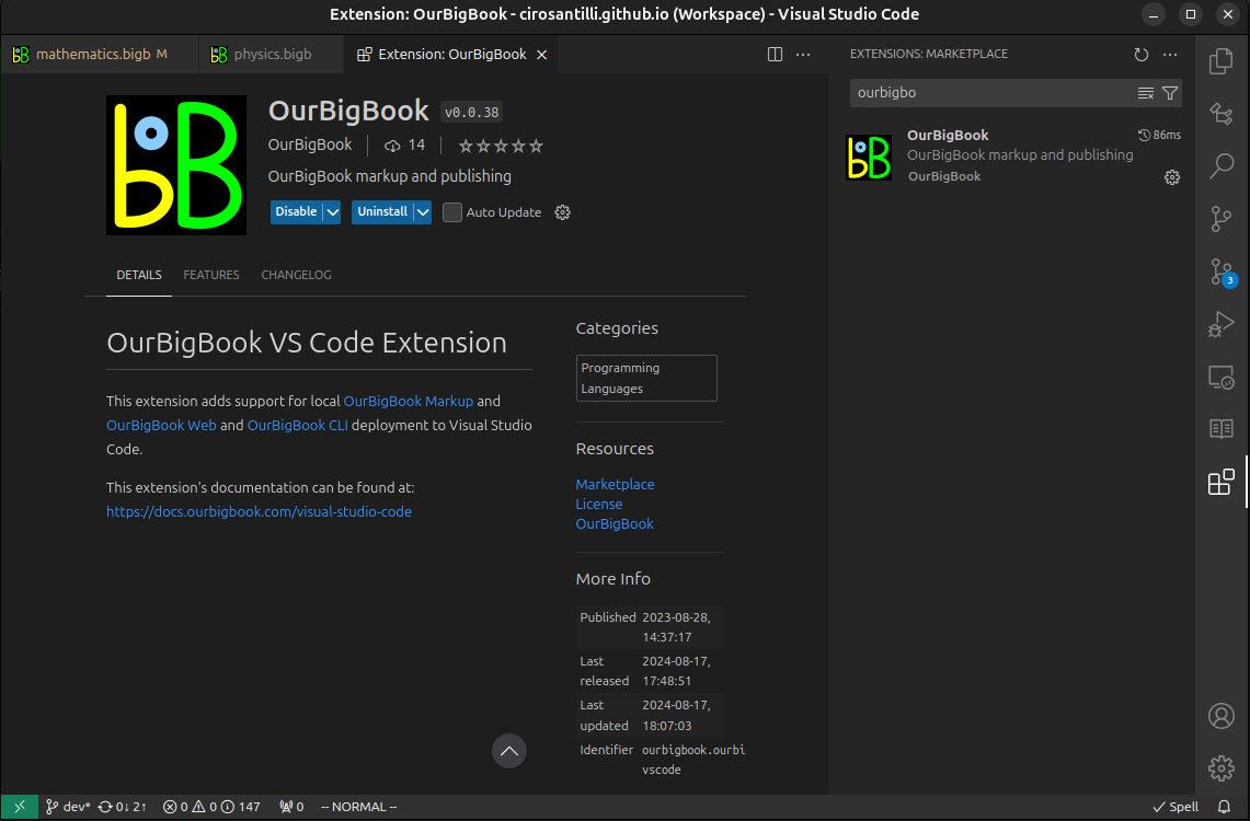
Figure 3. Visual Studio Code extension installation.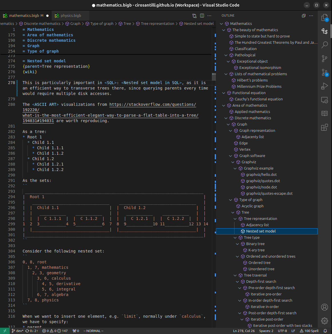
Figure 4. Visual Studio Code extension tree navigation.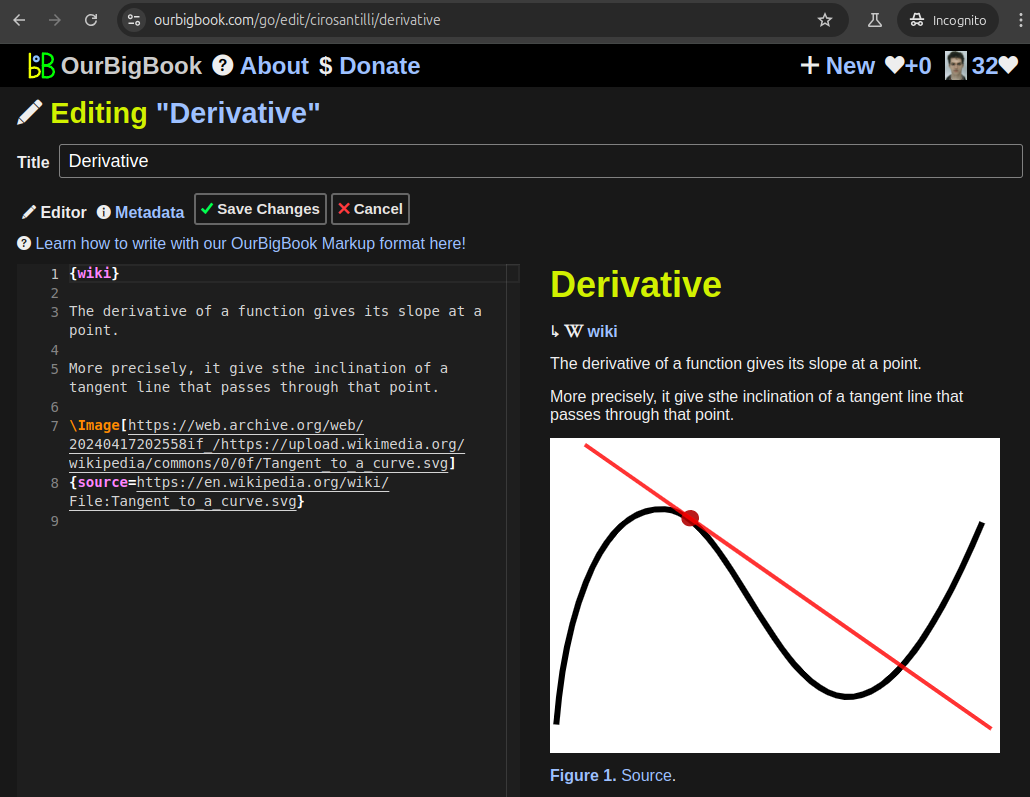
Figure 5. Web editor. You can also edit articles on the Web editor without installing anything locally.Video 3. Edit locally and publish demo. Source. This shows editing OurBigBook Markup and publishing it using the Visual Studio Code extension.Video 4. OurBigBook Visual Studio Code extension editing and navigation demo. Source. 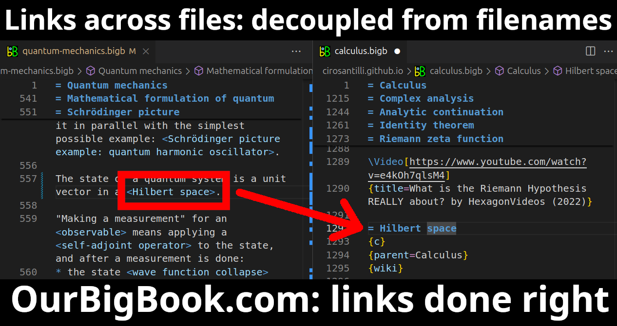
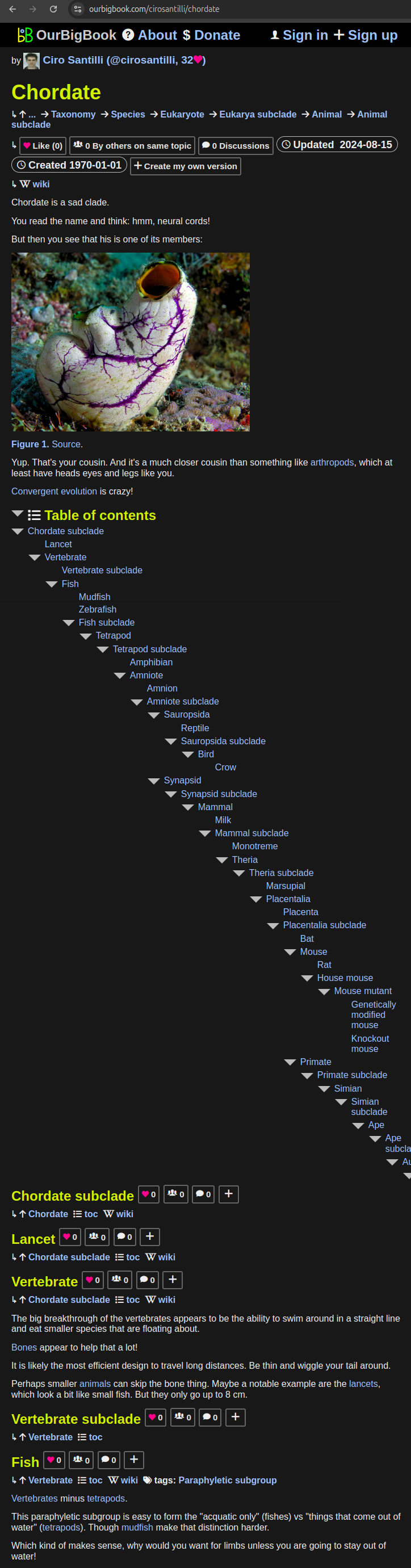
- Infinitely deep tables of contents:

All our software is open source and hosted at: github.com/ourbigbook/ourbigbook
Further documentation can be found at: docs.ourbigbook.com
Feel free to reach our to us for any help or suggestions: docs.ourbigbook.com/#contact