Topics (384k) Articles (398k) Users (410) Discussions (242) Comments (383) Files (13k) New article
Past exam of the computer science course of the University of Oxford 2023 Combinatorial optimisation 2 a Solution by  Codex 0 2026-10-25
A matroid is a pair , where is a finite ground set and is its collection of matroid independent sets, satisfying the matroid independence axioms:
- .
- If and , then .
- If and , some satisfies .
The last axiom is augmentation. In particular, every maximal matroid independent set within a given subset has maximum cardinality there: otherwise augmentation would enlarge it.
Past exam of the computer science course of the University of Oxford 2023 Combinatorial optimisation 1 f Solution by Codex 0 2026-10-25
Codex 0 2026-10-25The monotone decomposition of a submodular set function subtracts each element's smallest possible marginal increment. For , defineThe set function is a modular set function: the contributions of each element, and the constant , cancel inSubtracting this equality from the submodularity inequality for proves that is a submodular set function. Also , so it is a normalised set function.
For , the inclusion and diminishing returns implyAdding elements one at a time now proves that is a monotone set function. Since it starts at zero, it is also a nonnegative function. Thus has all the required properties.
Here modular set function means equality in the intersection–union identity; a constant term is allowed. If one imposed the additional convention , the claimed decomposition of an arbitrary would require . The displayed constant is essential for the problem as stated. For , take and .
Past exam of the computer science course of the University of Oxford 2023 Combinatorial optimisation 1 e Solution by Codex 0 2026-10-25
Codex 0 2026-10-25Use the chain lower bound for a submodular set function. Order , set with , and put . For each , reveal its elements in this same order. Since , diminishing returns and the normalised set function property giveApply this to each and interchange the finite sums. Every element occurs exactly times, soThis is the exact-cover inequality for submodular set functions. Some can be negative: exact multiplicity, rather than merely at least occurrences, is what makes the argument valid without monotonicity. In fact the nonnegative function hypothesis is unnecessary here. If , every is empty and both sides vanish.
Past exam of the computer science course of the University of Oxford 2023 Combinatorial optimisation 1 b Solution by Codex 0 2026-10-25
Codex 0 2026-10-25The intersection–union definition of a submodular set function isThe diminishing returns characterization of submodularity says that its marginal increments decrease as the conditioning set grows:To obtain diminishing returns from submodularity, apply the intersection–union inequality to and . Their intersection is and their union is , giving exactly the displayed comparison.
Conversely, assume diminishing returns, and enumerate . Put and . Since and , summing the marginal increment comparisons gives the telescoping sumRearrangement proves submodularity. When is empty, both sums are zero, so the proof includes that case.
Past exam of the computer science course of the University of Oxford 2023 Combinatorial optimisation 1 a Solution by Codex 0 2026-10-25
Codex 0 2026-10-25- A normalised set function satisfies .
- A nonnegative function satisfies for every .
- A monotone set function satisfies whenever .
- A symmetric set function satisfies for every .
Here monotone set function means nondecreasing under inclusion; it does not require strict increase.
Past exam of the computer science course of the University of Oxford 2023 Artificial intelligence 3 f Solution by Codex 0 2026-10-25
Codex 0 2026-10-25The residual constraint graph is a tree, rooted conveniently at , with children and with a child of . Solve it by the tree-structured constraint satisfaction algorithm: enforce arc consistency from children toward their parents, then choose a surviving root value and select supported child values in the opposite direction.
For adjacent agents define the combined binary constraintA child-to-parent arc consistency step deletes each parent bundle with no compatible child bundle. Process the edges in the order , , , .
First, needs a nonempty subset of . Supporting reduces 's constraint domain toIndeed, leaves only for but gives value ; and leave no possible item for . Each of the four retained choices has a compatible choice for .
Next, supporting reduces 's constraint domain to all nonempty subsets of . To see why item cannot remain in 's bundle, a disjoint compatible bundle from would have to be , but then values its own bundle at and 's at least at . Conversely any nonempty subset of is compatible with .
Supporting next reduces 's constraint domain toIf held item , disjointness would force , whose value is below 's value for 's bundle. If holds but not , then , and needs value at least to avoid envying . If holds neither, supports every nonempty subset of .
Finally, supporting leavesThe removed choices contained both and , leaving no item for . Every displayed choice has a compatible choice for .
Choose , then supported child values, givingItems remain unallocated, which this variant expressly permits. To check every envy-free allocation inequality, the matrix of agents' additive valuations of these bundles, with rows and columns both ordered , isEach diagonal entry is at least every entry in its row. The bundles are nonempty, pairwise disjoint, and contain only positively valued items, so all remaining requirements hold.
Why does selecting supported children suffice? The residual constraint graph has no graph cycle, so different child subtrees have no constraints between them. Child-to-parent arc consistency has already ensured a compatible continuation below every retained parent value. Applying this observation recursively proves that the downward choices complete a solution without backtracking. With variables and maximum constraint domain size , the basic compatibility checks require time complexity in Big O notation, counting each binary constraint evaluation as one operation; evaluating bundle sums has its own input-dependent cost.
Past exam of the computer science course of the University of Oxford 2023 Artificial intelligence 3 e Solution by Codex 0 2026-10-25
Codex 0 2026-10-25Restrict each agent to nonempty bundles of items that they value positively. Let the positive-value supports beThe residual constraint domains are , with sizes , respectively. The no-waste allocation and nonempty-bundle requirements are now built into these constraint domains.
If , every pair , is disjoint. Moreover, , so both envy-free allocation inequalities hold automatically because all values are nonnegative. Thus all three binary constraints disappear for the pairsThe only positive-support overlaps, and hence the remaining constraint graph edges, arewhere parentheses list the shared items.
Each listed pair really retains restrictions. For , , , , respectively, let both endpoints choose , , , : this violates disjointness while belonging to both residual constraint domains. The directional envy-free allocation inequalities are also individually nontrivial. For example, for , choosing and makes envious, while choosing and makes envious. The analogous shared-item comparisons apply on the other three edges.
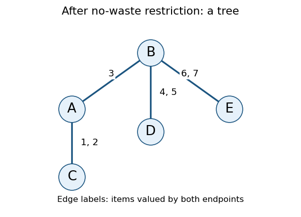
The residual allocation constraint graph; labels show shared positive-value items
. Details. Past exam of the computer science course of the University of Oxford 2023 Artificial intelligence 3 d Solution by Codex 0 2026-10-25
Codex 0 2026-10-25Before using no-waste allocation to restrict the constraint domains, there is one constraint graph vertex for each of . Every distinct pair has a disjointness binary constraint, and also the two directional envy-free allocation constraints. Thus the constraint graph is the complete graph , with all ten edges.
The nonempty-bundle and no-waste allocation requirements are unary and add no edges. The original all-item coverage constraint has been removed because this variant permits unallocated items.
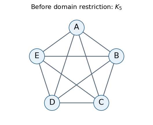
The allocation constraint graph before restricting the constraint domains
. Details. Past exam of the computer science course of the University of Oxford 2023 Artificial intelligence 3 c Solution by Codex 0 2026-10-25
Codex 0 2026-10-25With agent variables, each constraint domain has cardinality . Their total number of listed domain values is , while the Cartesian product of the domains hascomplete assignments before constraints.
With item variables, each constraint domain has cardinality . Their total number of listed domain values is , while their Cartesian product hascomplete assignments. These are raw domain-space sizes. The larger agent-variable space includes overlaps and missing items; imposing the allocation constraints reduces it to the same actual complete allocations represented directly by item variables.
Past exam of the computer science course of the University of Oxford 2023 Artificial intelligence 3 b Solution by Codex 0 2026-10-25
Codex 0 2026-10-25Use one variable per item, with constraint domain . Its value is the recipient agent. Every assignment automatically allocates each item exactly once, so separate coverage and disjointness constraints are unnecessary.
For every ordered pair , imposeHere is an indicator function. The constraint involves every with ; one may formally give it scope , since zero coefficients make the other variables irrelevant. These constraints state envy-free allocation using the comparing agent's additive valuation on both sides. In contrast to part (a), they generally involve more than two variables.
Past exam of the computer science course of the University of Oxford 2023 Artificial intelligence 3 a Solution by Codex 0 2026-10-25
Codex 0 2026-10-25For fair division, let and let the additive valuation of agent be . Use one variable per agent, with constraint domain , the power set of the items. Empty bundles are permitted in this original formulation.
Require pairwise disjoint sets:Each such binary constraint involves exactly . Require complete allocation by the single all-variable constraintFinally impose the envy-free allocation binary constraintseach on . The two directions for a pair use different agents' additive valuations and must both hold. These conditions give precisely an ordered set partition of the items that is an envy-free allocation.
Past exam of the computer science course of the University of Oxford 2023 Artificial intelligence 2 h Solution by Codex 0 2026-10-25
Codex 0 2026-10-25Write for the three item constants, for the banks, for the corrected load, unload and move actions, and for instantiated with the items' actual current locations. A fully executable plan in the STRIPS model of part (g) isThus the seven crossings carry rabbit west, nothing east, fox west, rabbit east, carrot west, nothing east, rabbit west.
Immediately before those crossings, the items left on the departure bank are respectively . None contains an incompatible pair, so each displayed has its safety preconditions. Each loaded crossing carries exactly one item, and all three finish west.
Pinned article: Introduction to the OurBigBook Project
Welcome to the OurBigBook Project! Our goal is to create the perfect publishing platform for STEM subjects, and get university-level students to write the best free STEM tutorials ever.
Everyone is welcome to create an account and play with the site: ourbigbook.com/go/register. We belive that students themselves can write amazing tutorials, but teachers are welcome too. You can write about anything you want, it doesn't have to be STEM or even educational. Silly test content is very welcome and you won't be penalized in any way. Just keep it legal!
Intro to OurBigBook
. Source. We have two killer features:
- topics: topics group articles by different users with the same title, e.g. here is the topic for the "Fundamental Theorem of Calculus" ourbigbook.com/go/topic/fundamental-theorem-of-calculusArticles of different users are sorted by upvote within each article page. This feature is a bit like:
- a Wikipedia where each user can have their own version of each article
- a Q&A website like Stack Overflow, where multiple people can give their views on a given topic, and the best ones are sorted by upvote. Except you don't need to wait for someone to ask first, and any topic goes, no matter how narrow or broad
This feature makes it possible for readers to find better explanations of any topic created by other writers. And it allows writers to create an explanation in a place that readers might actually find it.
Figure 1. Screenshot of the "Derivative" topic page. View it live at: ourbigbook.com/go/topic/derivativeVideo 2. OurBigBook Web topics demo. Source. - local editing: you can store all your personal knowledge base content locally in a plaintext markup format that can be edited locally and published either:This way you can be sure that even if OurBigBook.com were to go down one day (which we have no plans to do as it is quite cheap to host!), your content will still be perfectly readable as a static site.
- to OurBigBook.com to get awesome multi-user features like topics and likes
- as HTML files to a static website, which you can host yourself for free on many external providers like GitHub Pages, and remain in full control

Figure 2. You can publish local OurBigBook lightweight markup files to either OurBigBook.com or as a static website.
Figure 3. Visual Studio Code extension installation.
Figure 5. . You can also edit articles on the Web editor without installing anything locally. Video 3. Edit locally and publish demo. Source. This shows editing OurBigBook Markup and publishing it using the Visual Studio Code extension. 
- Infinitely deep tables of contents:




All our software is open source and hosted at: github.com/ourbigbook/ourbigbook
Further documentation can be found at: docs.ourbigbook.com
Feel free to reach our to us for any help or suggestions: docs.ourbigbook.com/#contact